코드
import pandas as pd
import numpy as np
import seaborn as sns
import matplotlib.pyplot as pltThis notebook presents an analysis of a dataset containing measurements of penguins. The goal is to investigate the existence of Simpson’s Paradox in the data.
Simpson’s Paradox is a phenomenon in probability and statistics, in which a trend appears in different groups of data but disappears or reverses when these groups are combined.
import pandas as pd
import numpy as np
import seaborn as sns
import matplotlib.pyplot as plt# Load the dataset
df = pd.read_csv('data/penguins.csv')# Check correlations within each species for culmen_length_mm and culmen_depth_mm
species_list = df['species'].unique()
for species in species_list:
print(f"Correlation within {species} species:")
print(df[df['species'] == species][['bill_length_mm', 'bill_depth_mm']].corr())
print("\n")Correlation within Adelie species:
bill_length_mm bill_depth_mm
bill_length_mm 1.000000 0.391492
bill_depth_mm 0.391492 1.000000
Correlation within Gentoo species:
bill_length_mm bill_depth_mm
bill_length_mm 1.000000 0.643384
bill_depth_mm 0.643384 1.000000
Correlation within Chinstrap species:
bill_length_mm bill_depth_mm
bill_length_mm 1.000000 0.653536
bill_depth_mm 0.653536 1.000000
# Calculate the overall correlation between bill_length_mm and bill_depth_mm
overall_corr = df[['bill_length_mm', 'bill_depth_mm']].corr().iloc[0, 1]
overall_corr-0.2350528703555336# Create a figure and axis
fig, ax = plt.subplots(figsize=(10, 8))
# Overall regression line
sns.regplot(x='bill_length_mm', y='bill_depth_mm', data=df, scatter=False,
line_kws={'color': 'black', 'label': "Overall regression line"})
# Loop through each species
for species in species_list:
species_data = df[df['species'] == species]
sns.scatterplot(x='bill_length_mm', y='bill_depth_mm', data=species_data, label=species)
sns.regplot(x='bill_length_mm', y='bill_depth_mm', data=species_data, scatter=False,
line_kws={'label': f"{species} regression line"})
plt.title('Bill Depth vs Bill Length')
plt.xlabel('Bill Length (mm)')
plt.ylabel('Bill Depth (mm)')
# Add legend
plt.legend()
plt.show()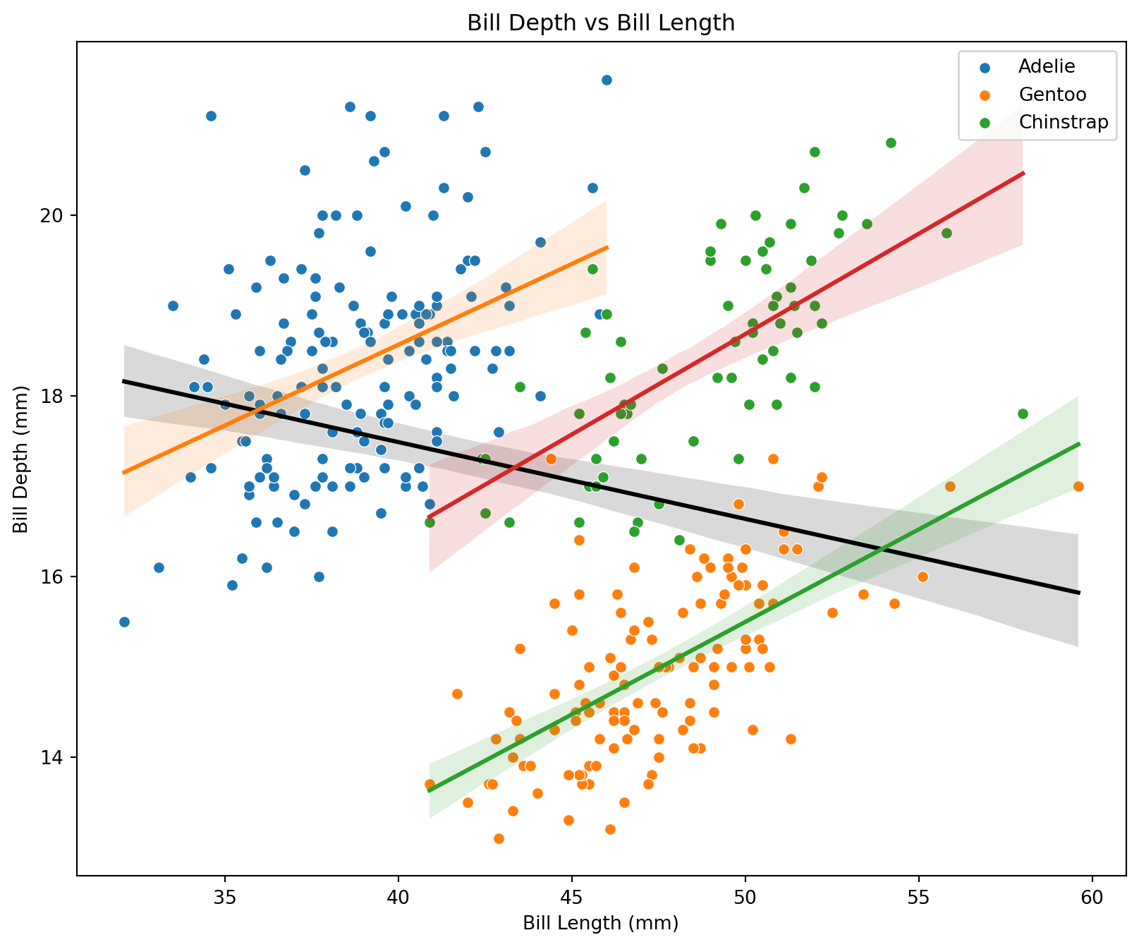
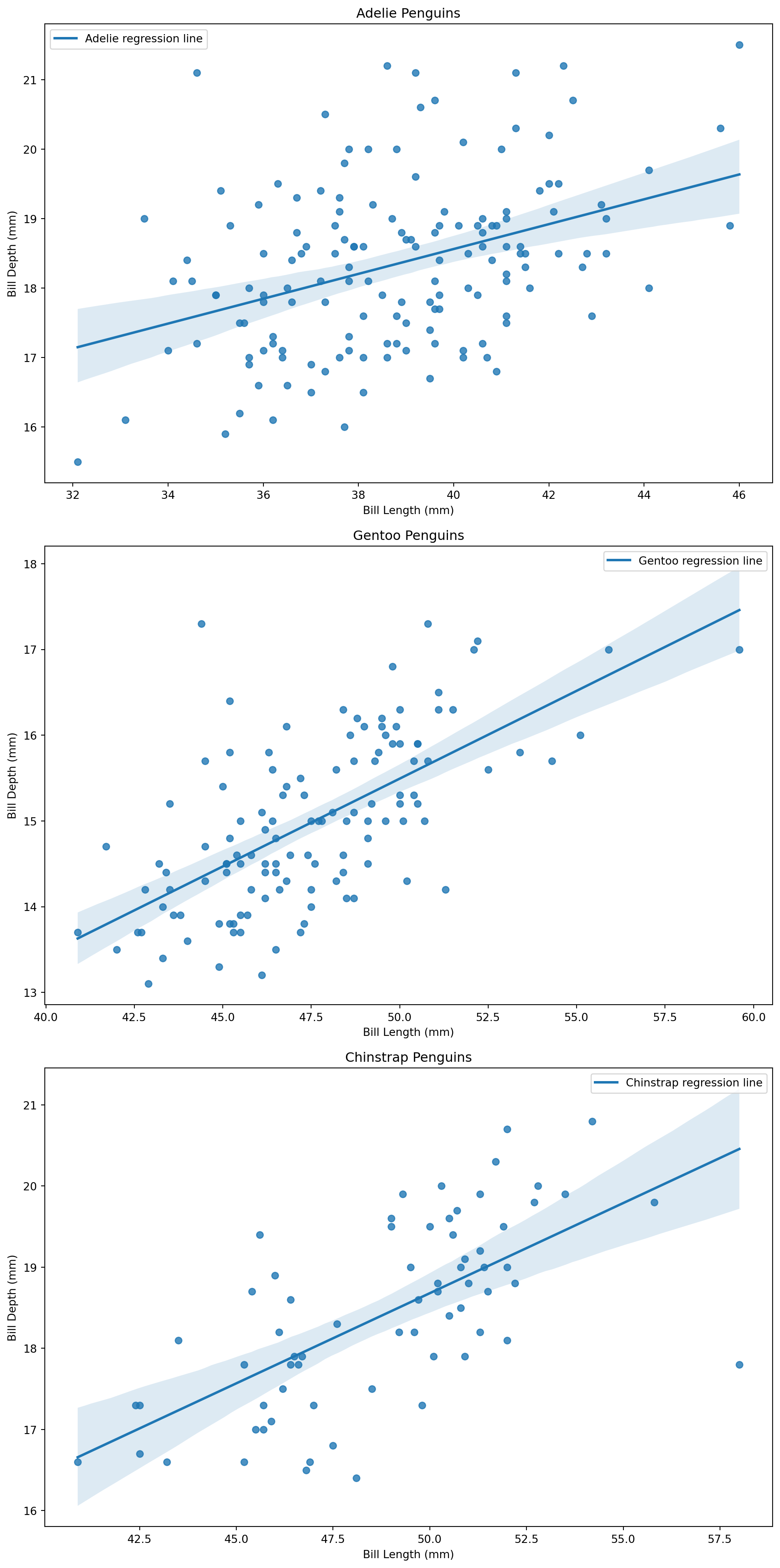
# Create a figure and axis
fig, axs = plt.subplots(3, 1, figsize=(10, 20))

# Loop through each species
for ax, species in zip(axs, species_list):
    species_data = df[df['species'] == species]
    sns.regplot(x='bill_length_mm', y='bill_depth_mm', data=species_data, ax=ax,
                line_kws={'label': f"{species} regression line"})
    ax.set_title(f'{species} Penguins')
    ax.set_xlabel('Bill Length (mm)')
    ax.set_ylabel('Bill Depth (mm)')
    ax.legend()

plt.tight_layout()
plt.show()