1 탐색적 데이터 분석
1.1 범주형 변수
범주형 변수(species, island, sex) 관계를 살펴보자.
1.1.1 species, island
species, island 시각화, 표, 검정 통계량을 통해 서로 독립이 아님이 확인된다.
– Adelie: 아델리 펭귄은 모든 섬에 서식 – Gentoo: 젠투 펭귄은 비스코(Biscoe) 섬에만 서식 – Chinstrap: 턱끈 펭귄은 드림(Dream) 섬에만 서식.
시각화
코드
penguins_colors <- c('#057076', '#ff8301', '#bf5ccb')

penguins %>%
  ggplot(aes(x = island, y = species, color = species)) +
  geom_jitter(size = 3) +
  scale_color_manual(values = penguins_colors)  +
  theme_bw(base_family = "NanumGothic") +
  theme(legend.position = "top") +
  labs(title = "펭귄종과 서식하는 섬",
       x = "섬",
y = "펭귄종명") 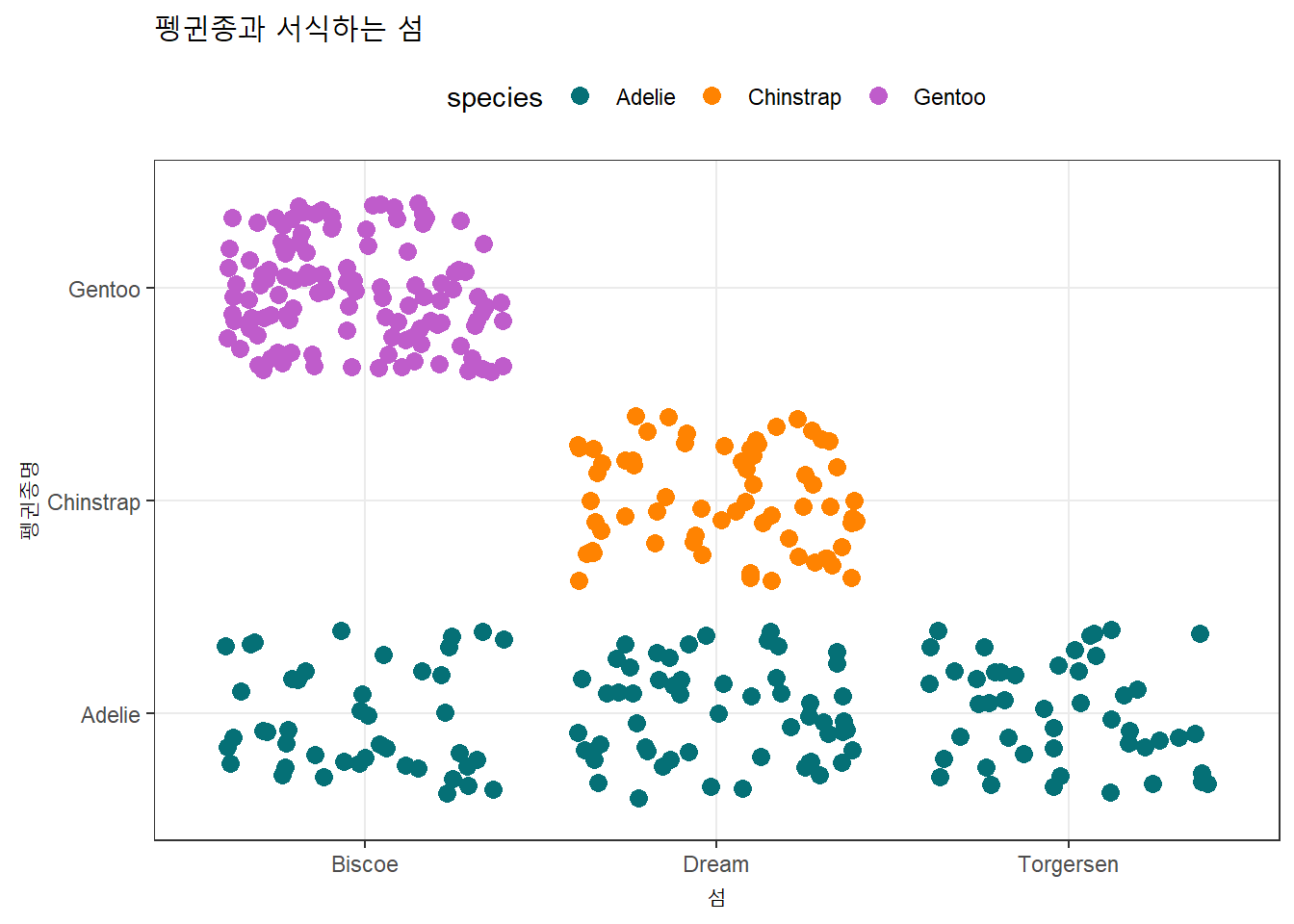
표
코드
library(gtExtras)

penguins %>%
  count(species, island) %>%
  pivot_wider(names_from = island, values_from = n, values_fill = 0) %>%
  gt::gt() %>%
gtExtras::gt_theme_538()| species | Biscoe | Dream | Torgersen |
|---|---|---|---|
| Adelie | 44 | 55 | 47 |
| Chinstrap | 0 | 68 | 0 |
| Gentoo | 119 | 0 | 0 |
통계검정
코드
library(infer)


# 관측통계량
observed_indep_statistic <- penguins %>%
  specify(species ~ island) %>%
  hypothesize(null = "independence") %>%
  calculate(stat = "Chisq")

# 통계검정 시각화
penguins %>%
  specify(species ~ island) %>%
  assume(distribution = "Chisq") %>%
  visualize() +
  shade_p_value(observed_indep_statistic,
direction = "greater") 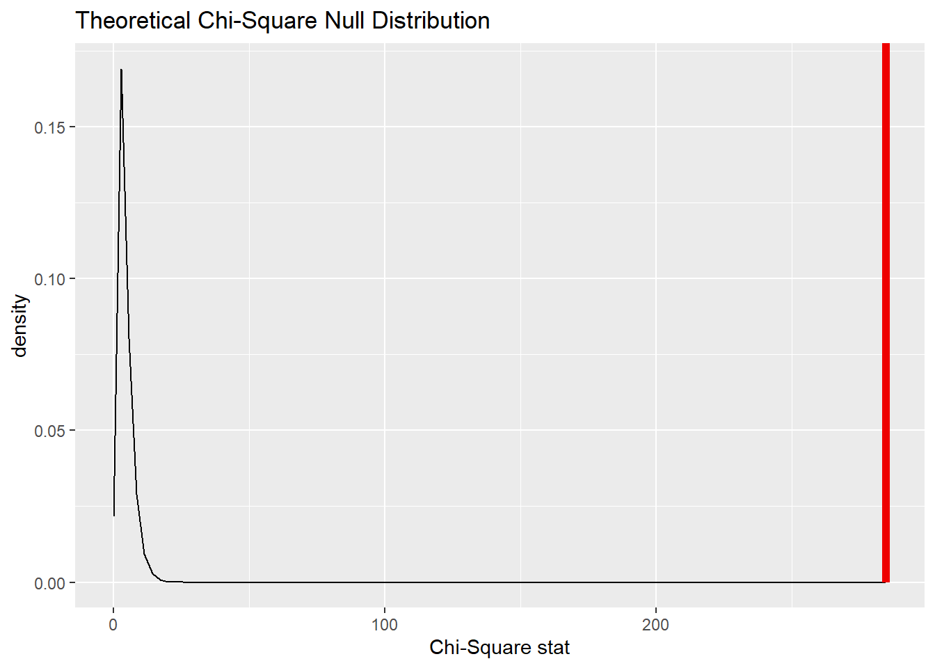
다른 species와 sex, sex와 island 범주 사이는 특별한 관계를 찾을 수 없음.
species와 sex
코드
library(janitor)
library(gt)

penguins %>%
  count(species, sex) %>%
  pivot_wider(names_from = sex, values_from = n, values_fill = 0) %>%
  adorn_totals("row", name = "합계") %>%
  adorn_percentages("row") %>%
  adorn_pct_formatting(digits = 1) %>%
  adorn_ns()  %>%
  gt::gt() %>%
  tab_options(table.font.names = 'NanumGothic',
                column_labels.font.weight = 'bold',
                heading.title.font.size = 14,
                heading.subtitle.font.size = 14,
                table.font.color = 'steelblue',
                source_notes.font.size = 10,
                #source_notes.
                table.font.size = 14) %>%
gtExtras::gt_theme_538()| species | female | male |
|---|---|---|
| Adelie | 50.0% (73) | 50.0% (73) |
| Chinstrap | 50.0% (34) | 50.0% (34) |
| Gentoo | 48.7% (58) | 51.3% (61) |
| 합계 | 49.5% (165) | 50.5% (168) |
sex와 island
코드
penguins %>%
  count(island, sex) %>%
  pivot_wider(names_from = sex, values_from = n, values_fill = 0) %>%
  adorn_totals("row", name = "합계") %>%
  adorn_percentages("row") %>%
  adorn_pct_formatting(digits = 1) %>%
  adorn_ns()  %>%
  gt::gt() %>%
tab_options(table.font.names = 'NanumGothic',
              column_labels.font.weight = 'bold',
              heading.title.font.size = 14,
              heading.subtitle.font.size = 14,
              table.font.color = 'darkgreen',
              source_notes.font.size = 10,
              #source_notes.
              table.font.size = 14) %>%
gtExtras::gt_theme_538()| island | female | male |
|---|---|---|
| Biscoe | 49.1% (80) | 50.9% (83) |
| Dream | 49.6% (61) | 50.4% (62) |
| Torgersen | 51.1% (24) | 48.9% (23) |
| 합계 | 49.5% (165) | 50.5% (168) |
1.2 연속형 변수
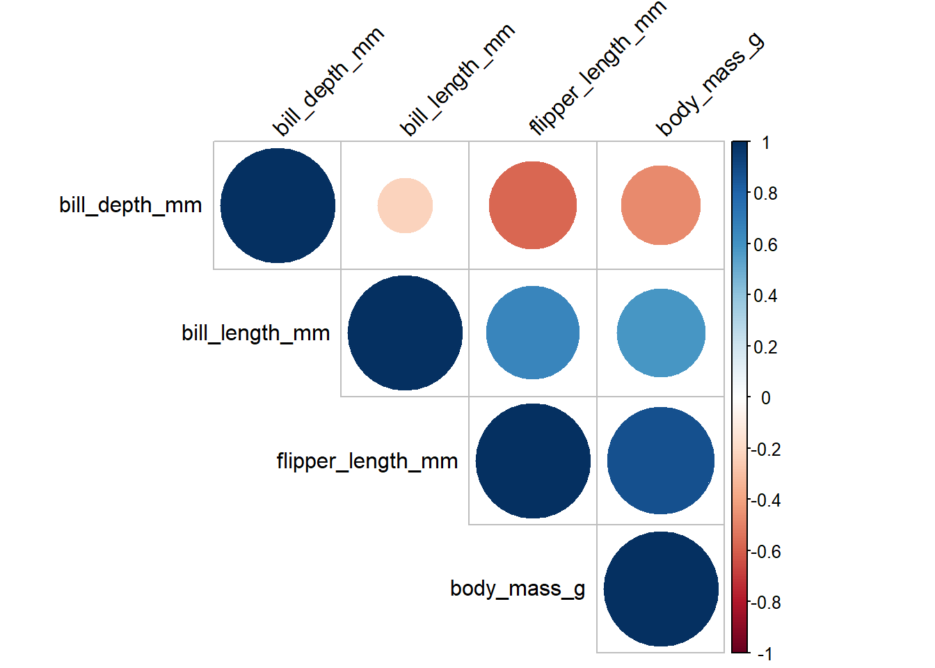
1.2.1 상관관계
penguins 데이터프레임에서 연속형 변수만 추출하여 상관관계를 살펴보자.
시각화
코드
상관계수 일반표
코드
library(corrr)
library(gt)

penguins_num %>%
  rename_with(.cols = everything(), .fn = ~str_remove(., pattern = "_mm|_g")) %>%
  corrr::correlate( use = "pairwise.complete.obs",
                    method = "pearson") %>%
  rearrange() %>%
  shave() %>%
  # fashion() %>%
  gt::gt() %>%
  # 상관계수 색상
  data_color(
    columns = where(is.numeric),
    colors = scales::col_numeric(
      ## option D for Viridis - correlation coloring
      palette = RColorBrewer::brewer.pal(9, "RdBu"),
      domain = NULL,
      na.color = 'white')
  ) %>%
  sub_missing(
    columns = everything(),
    missing_text = "-"
  ) %>%
  cols_align(align = "center", columns = everything()) %>%
gtExtras::gt_theme_538() | term | flipper_length | body_mass | bill_length | bill_depth |
|---|---|---|---|---|
| flipper_length | - | - | - | - |
| body_mass | 0.8729789 | - | - | - |
| bill_length | 0.6530956 | 0.5894511 | - | - |
| bill_depth | -0.5777917 | -0.4720157 | -0.2286256 | - |
상관계수 긴 표
코드
corrr::correlate(penguins_num) %>%
  stretch(remove.dups = TRUE) %>%
  filter(!is.na(r)) %>%
  arrange(desc(r)) %>%
  mutate(음양 = ifelse(r > 0, "양의 상관", "음의 상관")) %>%
  mutate(color = "") %>%
  gt(groupname_col = "음양") %>%
  fmt_number(
    columns = r,
    decimals = 2,
    use_seps = FALSE
  )  %>%
  data_color(
    columns = r,
    target_columns = color,
    method = "numeric",
    palette = RColorBrewer::brewer.pal(9, "RdBu")
  ) %>%
  cols_label(
    x = "",
    y = "",
    r = "상관계수",
    color = ""
  ) |>
  opt_vertical_padding(scale = 0.7)  %>%
gtExtras::gt_theme_538()| 상관계수 | |||
|---|---|---|---|
| 양의 상관 | |||
| flipper_length_mm | body_mass_g | 0.87 | |
| bill_length_mm | flipper_length_mm | 0.65 | |
| bill_length_mm | body_mass_g | 0.59 | |
| 음의 상관 | |||
| bill_length_mm | bill_depth_mm | −0.23 | |
| bill_depth_mm | body_mass_g | −0.47 | |
| bill_depth_mm | flipper_length_mm | −0.58 | |
1.2.2 평행 그래프
코드
library(GGally)

penguins %>%
  select(species, bill_length_mm, bill_depth_mm, flipper_length_mm, body_mass_g) %>%
  ggparcoord(columns = 2:5,
             showPoints = TRUE,
             groupColumn = "species") +
  scale_color_manual(values = penguins_colors)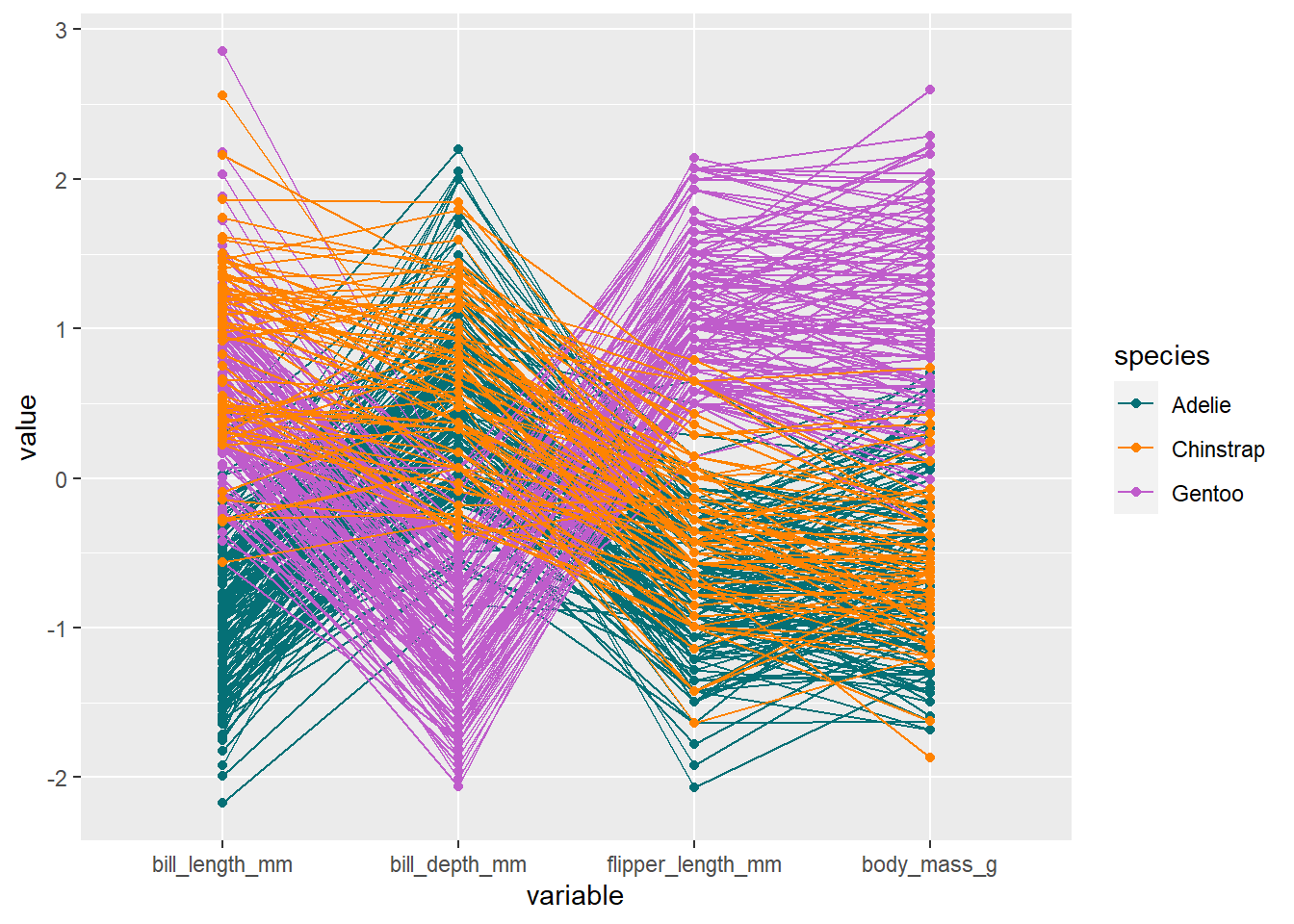
1.2.3 짝 산점도
코드
penguins %>%
  select(species, bill_length_mm, bill_depth_mm, flipper_length_mm, body_mass_g) %>%
  ggpairs(columns = 2:5, ggplot2::aes(colour=species),
          upper = list(continuous='density', combo='box_no_facet'),
          axisLabels='internal') +
  scale_color_manual(values = penguins_colors) +
  scale_fill_manual(values = penguins_colors) +
  theme_minimal()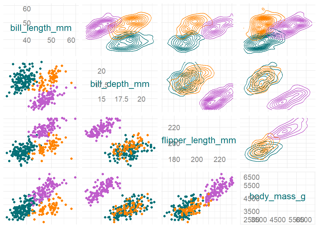
2 모형
2.1 성별 분류모형
펭귄의 암수를 분류하는 기계학습모형을 개발하기 전에 훈련/시험 데이터셋으로 나눈다.
코드
library(tidymodels)

penguins_split <- penguins %>%
  initial_split(prop = 0.70, strata = sex)

penguins_train <- training(penguins_split)
penguins_test  <- testing(penguins_split)
2.1.1 로지스틱 회귀
펭귄의 암수를 분류하는 로지스틱 회귀모형으로 분류모형을 개발해보자.
코드
logistic_spec <- logistic_reg() %>%
  set_engine("glm") %>%
  set_mode("classification")

logistic_wflow <-
  workflow(
    sex ~ species + island + bill_length_mm + bill_depth_mm +
          flipper_length_mm + body_mass_g,
    logistic_spec
  )

logistic_fit <- logistic_wflow %>% fit(data = penguins_train)

sex_predict <- predict(logistic_fit, penguins_test, type = "class")

bind_cols(penguins_test, sex_predict) %>%
  ggplot(aes(x = sex, y = .pred_class, color = sex)) +
  geom_jitter(size = 1, width = 0.2, height = 0.2) +
  scale_color_manual(values = c("blue", "red")) +
  theme_bw()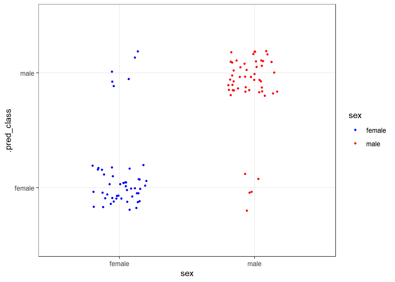
2.1.2 Random Forest
펭귄의 암수를 분류하는 Random Forest 모형으로 분류모형을 개발해보자.
코드
rf_spec <- rand_forest() %>%
  set_engine("ranger") %>%
  set_mode("classification")

rf_wflow <-
  workflow(
    sex ~ species + island + bill_length_mm + bill_depth_mm +
          flipper_length_mm + body_mass_g,
    rf_spec
  )

rf_fit <- rf_wflow %>% fit(data = penguins_train)

sex_rf <- predict(rf_fit, penguins_test, type = "class")

bind_cols(penguins_test, sex_rf) %>%
  ggplot(aes(x = sex, y = .pred_class, color = sex)) +
  geom_jitter(size = 1, width = 0.2, height = 0.2) +
  scale_color_manual(values = c("blue", "red")) +
  theme_bw()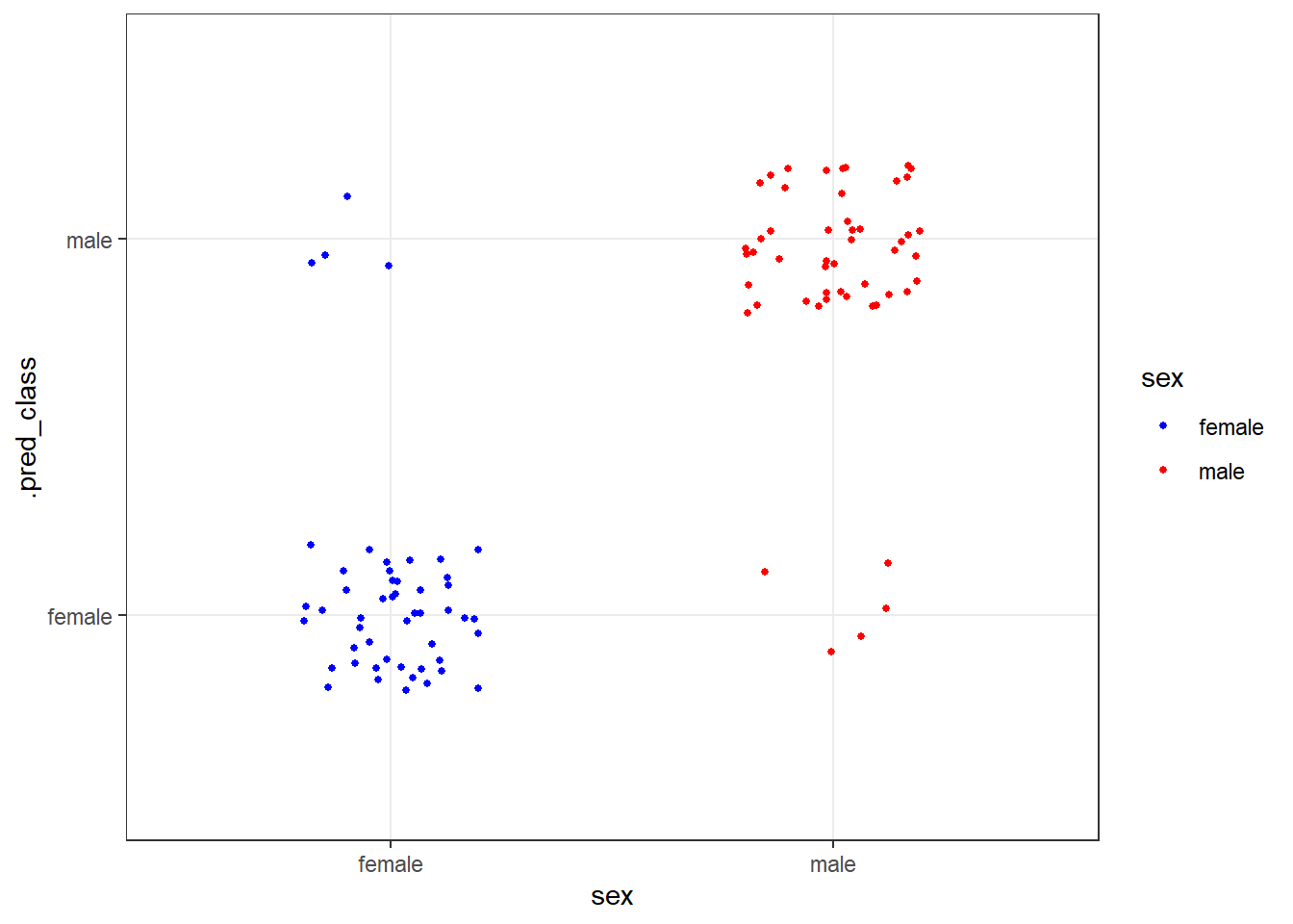
2.1.3 SVM
펭귄의 암수를 분류하는 SVM 모형으로 분류모형을 개발해보자.
코드
svm_spec <- svm_rbf() %>%
  set_engine("kernlab") %>%
  set_mode("classification")

svm_wflow <-
  workflow(
    sex ~ species + island + bill_length_mm + bill_depth_mm +
          flipper_length_mm + body_mass_g,
    svm_spec
  )

svm_fit <- svm_wflow %>% fit(data = penguins_train)

sex_svm <- predict(svm_fit, penguins_test, type = "class")

bind_cols(penguins_test, sex_svm) %>%
  ggplot(aes(x = sex, y = .pred_class, color = sex)) +
  geom_jitter(size = 1, width = 0.2, height = 0.2) +
  scale_color_manual(values = c("blue", "red")) +
  theme_bw()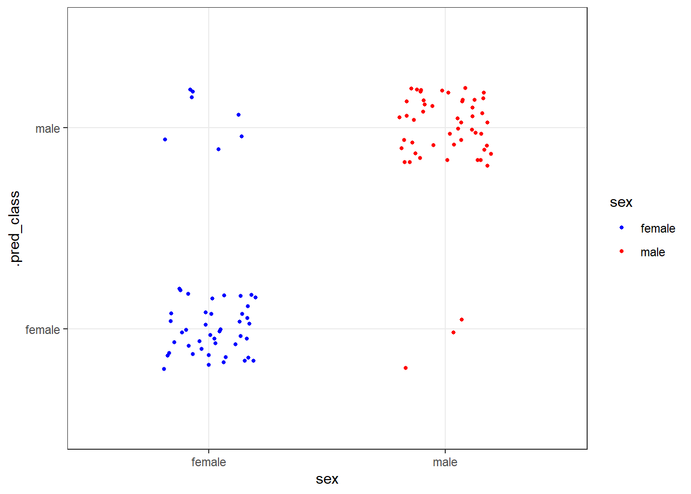
2.2 펭귄종 분류모형
펭귄종(아델리, 젠투, 턱끈)을 분류하는 기계학습모형을 개발하기 전에 훈련/시험 데이터셋으로 나눈다.
2.2.1 다항회귀모형
펭귄종(아델리, 젠투, 턱끈)을 분류하는 로지스틱 회귀모형으로 분류모형을 개발해보자.
코드
multinom_spec <- multinom_reg() %>%
  set_mode("classification")

multinom_wflow <-
  workflow(
    species ~ sex + island + bill_length_mm + bill_depth_mm +
          flipper_length_mm + body_mass_g,
    multinom_spec
  )

multinom_fit <- multinom_wflow %>% fit(data = penguins_train)

sex_predict <- predict(multinom_fit, penguins_test, type = "class")

bind_cols(penguins_test, sex_predict) %>%
  ggplot(aes(x = species, y = .pred_class, color = species)) +
  geom_jitter(size = 1, width = 0.2, height = 0.2) +
  scale_color_manual(values = penguins_colors) +
  theme_bw()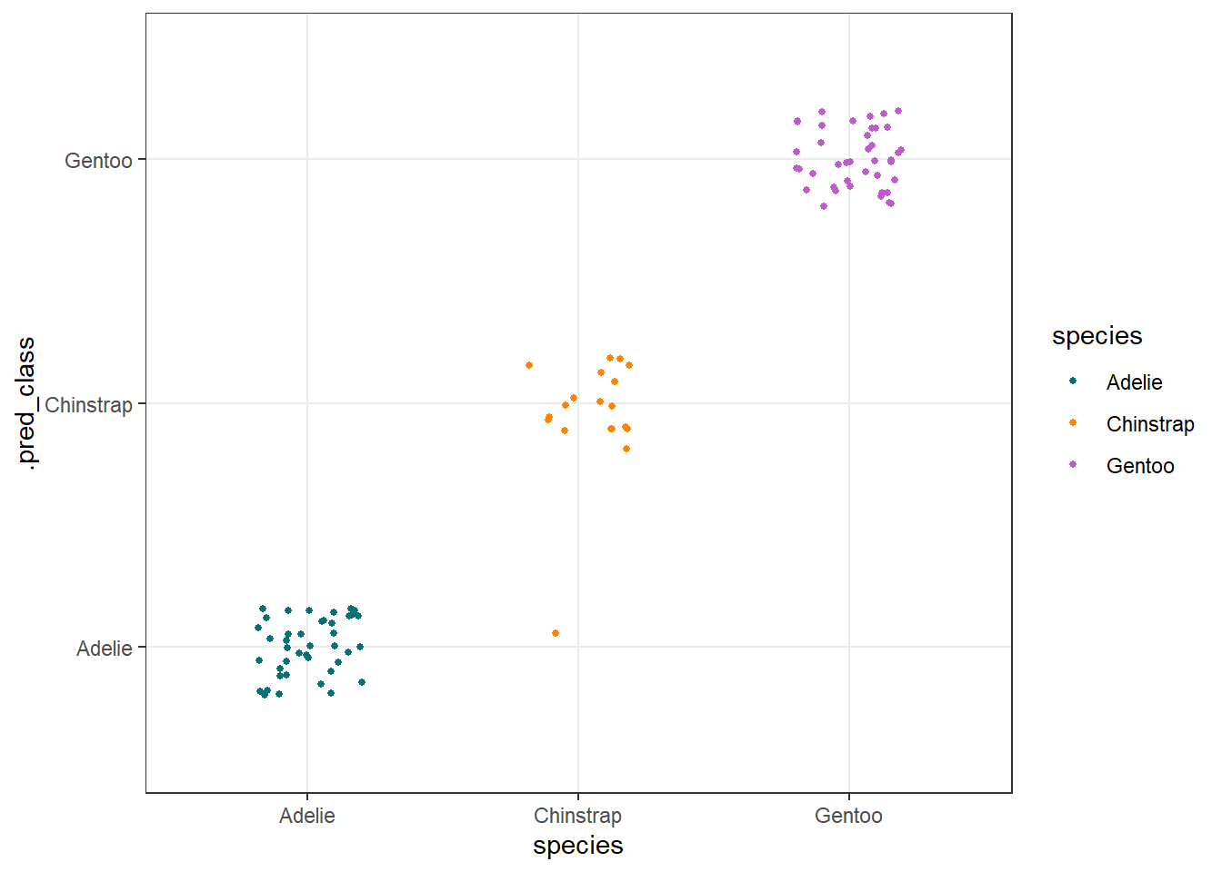
2.2.2 Random Forest
펭귄종(아델리, 젠투, 턱끈)을 분류하는 Random Forest 모형으로 분류모형을 개발해보자.
코드
rf_spec <- rand_forest() %>%
  set_engine("ranger") %>%
  set_mode("classification")

rf_wflow <-
  workflow(
    species ~ sex + island + bill_length_mm + bill_depth_mm +
          flipper_length_mm + body_mass_g,
    rf_spec
  )

rf_fit <- rf_wflow %>% fit(data = penguins_train)

sex_rf <- predict(rf_fit, penguins_test, type = "class")

bind_cols(penguins_test, sex_rf) %>%
  ggplot(aes(x = species, y = .pred_class, color = species)) +
  geom_jitter(size = 1, width = 0.2, height = 0.2) +
  scale_color_manual(values = penguins_colors) +
  theme()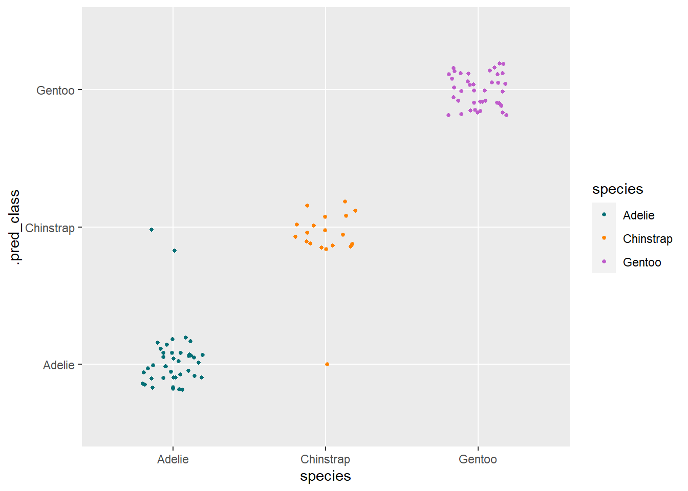
3 고급 시각화
3.1 펭귄크기와 물칼퀴
코드
extrafont::loadfonts()
ggplot2::theme_set(ggplot2::theme_minimal(base_family = "MaruBuri"))

species_mean <- penguins %>%
  group_by(species) %>%
  summarise(flipper_mean = mean(flipper_length_mm),
         body_mass_mean  = mean(body_mass_g))

penguins %>%
  ggplot(aes(x = flipper_length_mm, y = body_mass_g)) +
  geom_point(aes(color = species, shape = species),
             size = 3, alpha = 0.8) +
  # 평균 추가
  geom_point(data = species_mean, aes(x = flipper_mean, y = body_mass_mean, shape = species),
             size = 5, color = "black", show.legend = FALSE) +
  scale_color_manual(values = c("darkorange", "purple", "cyan4")) +
  labs(title = "남국 파머 연구수 서식 펭귄 크기",
       subtitle = "아델리, 젠투, 턱끈 펭귄 물갈퀴 길이와 체질량",
       x = "물갈퀴 길이 (mm)",
       y = "체질량 (g)",
       color = "펭귄종",
       shape = "펭귄종") +
  theme(legend.position = c(0.9, 0.2),
        plot.title.position = "plot",
        plot.caption = element_text(hjust = 0, face= "italic"),
plot.caption.position = "plot") 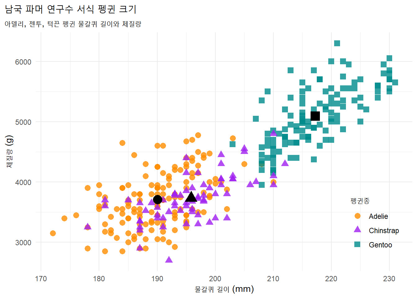
3.2 물갈퀴와 부리 길이
코드
species_mean <- penguins %>%
  group_by(species) %>%
  summarise(flipper_mean = mean(flipper_length_mm),
            bill_mean  = mean(bill_length_mm))

penguins %>%
  ggplot(aes(x = flipper_length_mm, y = bill_length_mm)) +
  geom_point(aes(color = species, shape = species),
             size = 3, alpha = 0.8) +
  # 평균 추가
  geom_point(data = species_mean, aes(x = flipper_mean, y = bill_mean, shape = species),
             size = 5, color = "black", show.legend = FALSE) +
  scale_color_manual(values = c("darkorange", "purple", "cyan4")) +
  labs(title = "물갈퀴 길이와 부리 길이",
       subtitle = "아델리, 젠투, 턱끈 펭귄 물갈퀴 길이와 부리 길이 치수",
       x = "물갈퀴 길이 (mm)",
       y = "부리 길이 (mm)",
       color = "펭귄종",
       shape = "펭귄종") +
  theme(legend.position = c(0.9, 0.2),
        plot.title.position = "plot",
        plot.caption = element_text(hjust = 0, face= "italic"),
plot.caption.position = "plot") 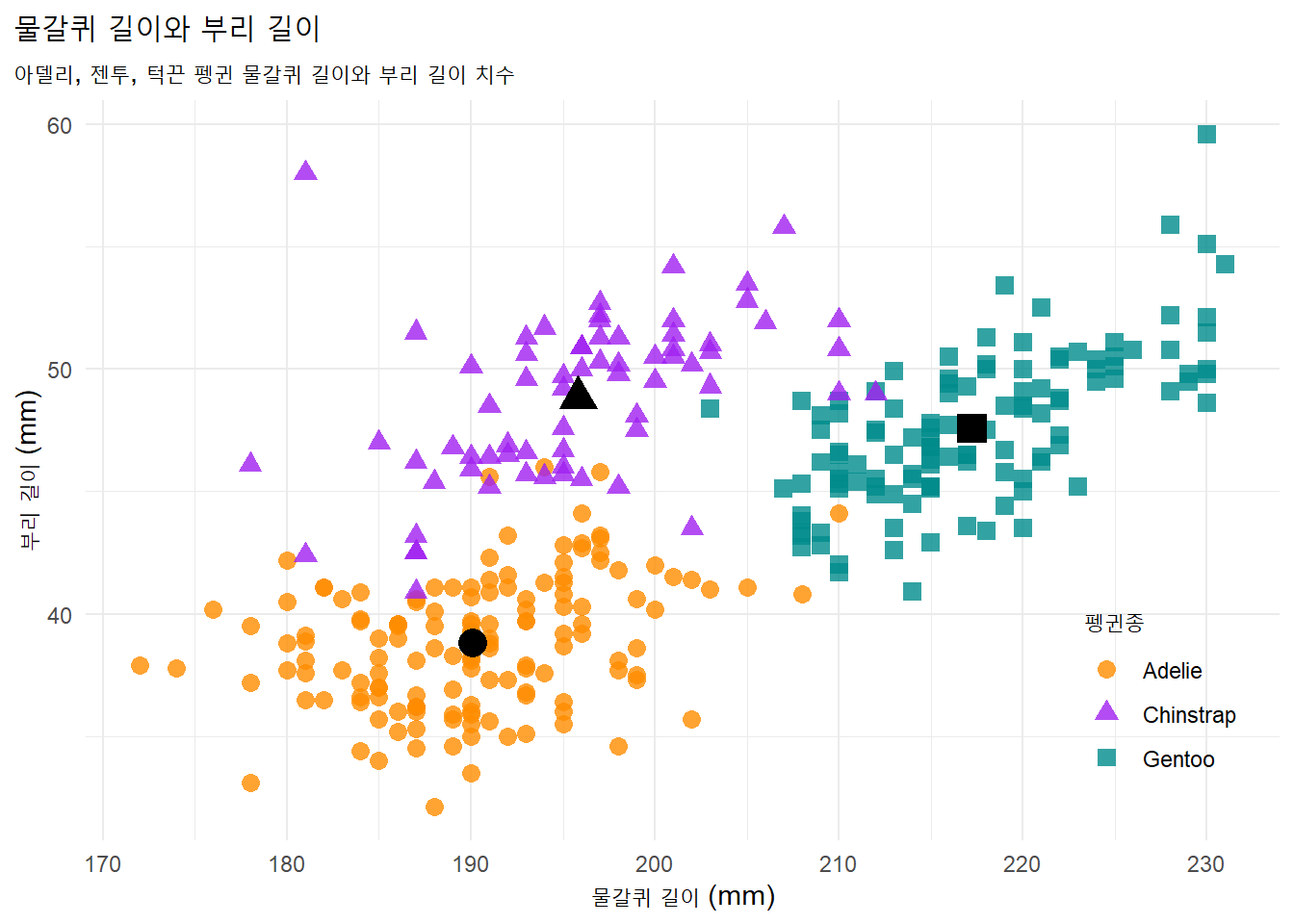
3.3 분포와 Facet
코드
ggplot(data = penguins, aes(x = flipper_length_mm)) +
  geom_histogram(aes(fill = species),
                 alpha = 0.5,
                 position = "identity") +
  scale_fill_manual(values = c("darkorange","purple","cyan4")) +
  labs(x = "물갈퀴 길이 (mm)",
       y = "빈도수",
       title = "펭귄 물갈퀴 길이",
       fill = "펭귄종")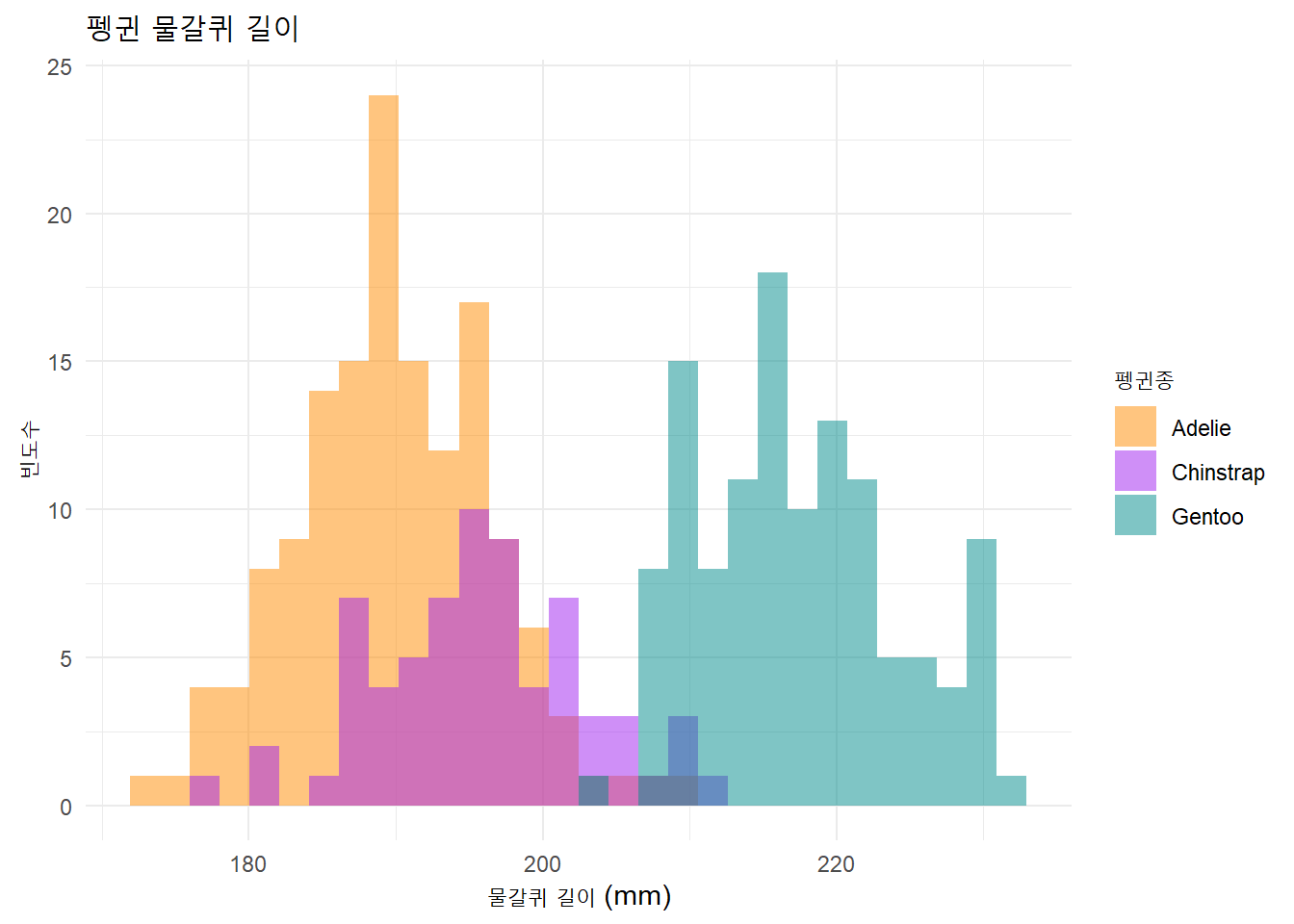
코드
ggplot(data = penguins, aes(x = species, y = flipper_length_mm)) +
  geom_boxplot(aes(color = species), width = 0.3, show.legend = FALSE) +
  geom_jitter(aes(color = species), alpha = 0.5, show.legend = FALSE,
              position = position_jitter(width = 0.2, seed = 0)) +
  scale_color_manual(values = c("darkorange","purple","cyan4")) +
  labs(x = "펭귄종",
       y = "물갈퀴 길이 (mm)",
       title = "펭귄종별 물갈퀴 길이 분포")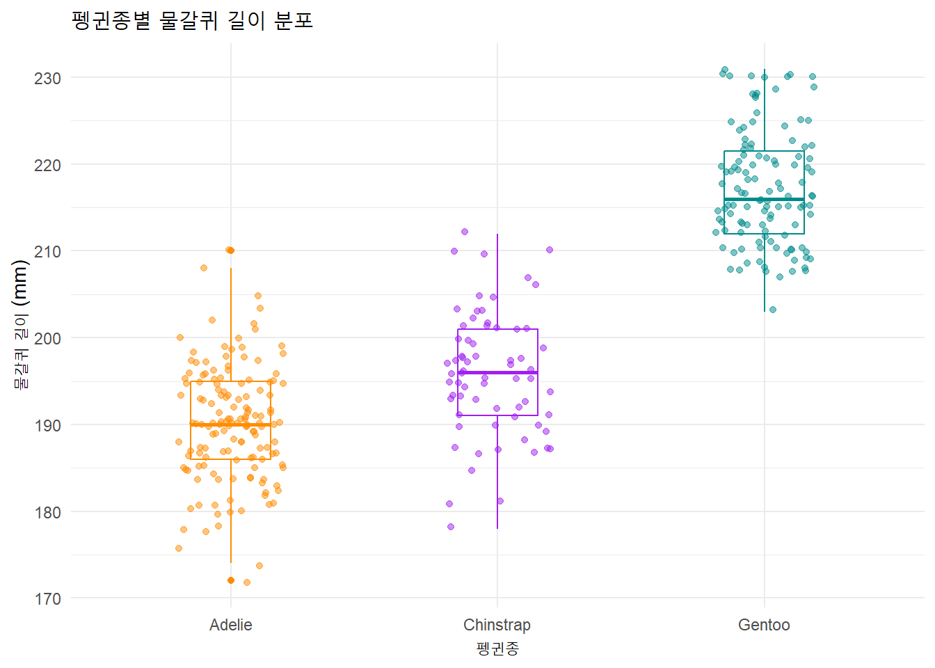
코드
ggplot(penguins, aes(x = flipper_length_mm, y = body_mass_g)) +
  geom_point(aes(color = sex)) +
  scale_color_manual(values = c("darkorange","cyan4"), na.translate = FALSE) +
  labs(title = "펭귄 물갈퀴 길이와 체질량",
       subtitle = "아델리, 젠투, 턱끈 펭귄 물갈퀴 길이와 체질량",
       x = "물갈퀴 길이 (mm)",
       y = "체질량 (g)",
       color = "펭귄암수") +
  theme(legend.position = "bottom",
        plot.title.position = "plot",
        plot.caption = element_text(hjust = 0, face= "italic"),
        plot.caption.position = "plot") +
  facet_wrap(~species)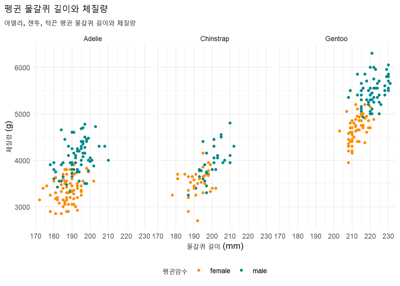
4 심슨 역설
심슨의 역설(Simpson’s Paradox)은 데이터를 취합할 때 의미 있는 변수를 생략하면 변수 간에 관찰되는 추세가 역전되는 데이터 현상이다.
부리의 길이와 깊이는 전체적으로 음의 상관관계를 보이지만, 종을 포함하면 이러한 추세가 반전되어 종 내에서는 부리 길이와 부리 깊이 사이에 양의 상관관계가 뚜렷하게 나타난다.
펭귄종 누락 시각화
코드
library(ggpubr)

penguins %>%
  ggplot(aes(x = bill_length_mm, y = bill_depth_mm)) +
    geom_point(size = 3, alpha = 0.8) +
    labs(title = "펭귄종을 누락한 상태 부리 길이와 깊이",
         subtitle = "남극 파머 연구소",
         x = "부리 길이 (mm)",
         y = "부리 깊이 (mm)") +
    theme(plot.title.position = "plot",
          plot.caption = element_text(hjust = 0, face= "italic"),
          plot.caption.position = "plot") +
    geom_smooth(method = "lm", se = FALSE, color = "gray50") +
    stat_regline_equation(label.x = 30, label.y = 22)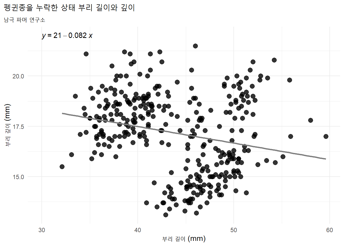
펭귄종 포함 시각화
코드
library(ggpmisc)

penguins %>%
  ggplot(aes(x = bill_length_mm, y = bill_depth_mm,
             color = species, shape = species)) +
    geom_point(size = 3, alpha = 0.8) +
    scale_color_manual(values = c("darkorange","purple","cyan4")) +
    stat_poly_line(formula = y ~ x, se = FALSE) +
    stat_poly_eq(aes(label = after_stat(eq.label)), formula = y ~ x) +
    labs(title = "펭귄종을 포함한 상태 부리 길이와 깊이",
         subtitle = "남극 파머 연구소",
         x = "부리 길이 (mm)",
         y = "부리 깊이 (mm)") +
    theme(plot.title.position = "plot",
          plot.caption = element_text(hjust = 0, face= "italic"),
          plot.caption.position = "plot",
legend.position = "top") 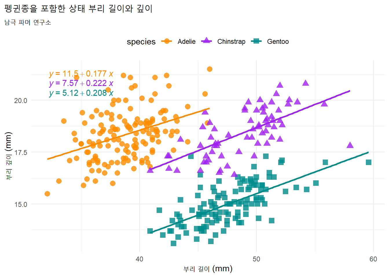
5 다변량 분석
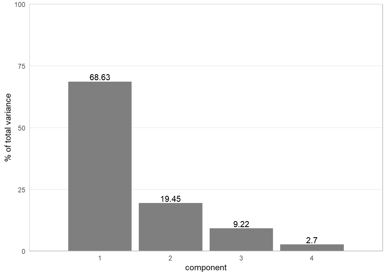
5.1 주성분 분석
주성분 분석(PCA)은 다변량 데이터의 패턴을 탐색하는 데 일반적으로 사용되는 차원 축소 방법이다. (Allison M. Horst, 2022)
코드
# Omit year
penguins_noyr <- penguins %>%
  select(-year) %>%
  mutate(species = as.character(species)) %>%
  mutate(species = case_when(
    species == "Adelie" ~ "Adélie",
    TRUE ~ species
  )) %>%
  mutate(species = as.factor(species))

penguin_recipe <-
  recipe(~., data = penguins_noyr) %>%
  update_role(species, island, sex, new_role = "id") %>%
  step_naomit(all_predictors()) %>%
  step_normalize(all_predictors()) %>%
  step_pca(all_predictors(), id = "pca") %>%
  prep()

penguin_pca <-
  penguin_recipe %>%
  tidy(id = "pca")

penguin_percvar <- penguin_recipe %>%
  tidy(id = "pca", type = "variance") %>%
  dplyr::filter(terms == "percent variance")

# Make the penguins PCA biplot:

# Get pca loadings into wider format
pca_wider <- penguin_pca %>%
  tidyr::pivot_wider(names_from = component, id_cols = terms)

# define arrow style:
arrow_style <- arrow(length = unit(.05, "inches"),
                     type = "closed")

penguins_juiced <- juice(penguin_recipe)

# Make the penguins PCA biplot:
pca_plot <-
  penguins_juiced %>%
  ggplot(aes(PC1, PC2)) +
  coord_cartesian(
    xlim = c(-3, 4),
    ylim = c(-2.5, 2))  +
  paletteer::scale_color_paletteer_d("colorblindr::OkabeIto") +
  guides(color = guide_legend("Species"),
        shape = guide_legend("Species")) +
  theme(legend.position = "bottom",
        panel.border = element_rect(color = "gray70", fill = NA))

# For positioning (above):
# 1: bill_length
# 2: bill_depth
# 3: flipper length
# 4: body mass

penguins_biplot <- pca_plot +
  geom_segment(data = pca_wider,
               aes(xend = PC1, yend = PC2),
               x = 0,
               y = 0,
               arrow = arrow_style) +
  geom_point(aes(color = species, shape = species),
             alpha = 0.7,
             size = 2) +
  shadowtext::geom_shadowtext(data = pca_wider,
                  aes(x = PC1, y = PC2, label = terms),
                  nudge_x = c(0.7,0.7,1.7,1.2),
                  nudge_y = c(-0.1,-0.2,0.1,-0.1),
                  size = 4,
                  color = "black",
                  bg.color = "white")

penguins_biplot

penguin_screeplot_base <- penguin_percvar %>%
  ggplot(aes(x = component, y = value)) +
  scale_x_continuous(limits = c(0, 5), breaks = c(1,2,3,4), expand = c(0,0)) +
  scale_y_continuous(limits = c(0,100), expand = c(0,0)) +
  ylab("% of total variance") +
  theme(panel.border = element_rect(color = "gray70", fill = NA),
        panel.grid.major.x = element_blank(),
        panel.grid.minor.x = element_blank(),
        panel.grid.minor.y = element_blank())

penguin_screeplot <- penguin_screeplot_base +
  geom_col(fill = "gray50") +
  geom_text(aes(label = round(value,2)), vjust=-0.25)

penguin_screeplot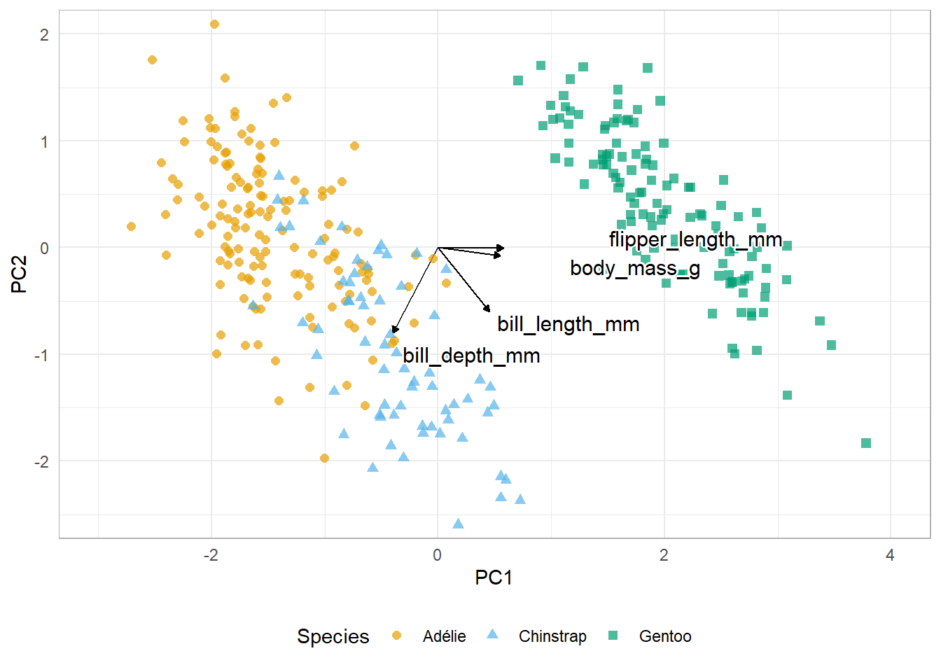
5.2 군집분석
k-평균(K-Means) 비지도학습 군집분석은 기계학습 및 분류에 대한 일반적이고 인기 있는 알고리즘이다.
코드
## ---- kmeans ---------------------------------------------------------

# TWO VARIABLE k-means comparison
# Penguins: Bill length vs. bill depth
pb_species <- penguins %>%
  select(species, starts_with("bill")) %>%
  drop_na() %>%
  mutate(species = as.character(species)) %>%
  mutate(species = case_when(
    species == "Adelie" ~ "Adélie",
    TRUE ~ species
  )) %>%
  mutate(species = as.factor(species))

# Prep penguins for k-means:
pb_nospecies <- pb_species %>%
  select(-species) %>%
  recipe() %>%
  step_normalize(all_numeric()) %>%
  prep() %>%
  juice()

# Perform k-means on penguin bill dimensions (k = 3, w/20 centroid starts)

# Save augmented data
set.seed(100)
pb_clust <-
  pb_nospecies %>%
  kmeans(centers = 3, nstart = 20) %>%
  broom::augment(pb_species)

# Get counts in each cluster by species
pb_clust_n <- pb_clust %>%
  count(species, .cluster) %>%
  pivot_wider(names_from = species, values_from = n, names_sort = TRUE) %>%
  arrange(.cluster) %>%
  replace_na(list(`Adelie` = 0))

# Plot penguin k-means clusters:
# make a base plot b/c https://github.com/plotly/plotly.R/issues/1942
pb_kmeans_base <-
  pb_clust %>%
  ggplot(aes(x = bill_length_mm, y = bill_depth_mm)) +
  paletteer::scale_color_paletteer_d("colorblindr::OkabeIto") +
  paletteer::scale_fill_paletteer_d("colorblindr::OkabeIto") +
  scale_x_continuous(limits = c(30, 60),
                     breaks = c(30, 40, 50, 60)) +
  theme(legend.position = "bottom",
        panel.border = element_rect(fill = NA, color = "gray70")) +
  labs(x = "Bill length (mm)",
       y = "Bill depth (mm)",
       color = "Species")
# ggpubr::stat_chull(aes(fill = .cluster, color = .cluster),
# alpha = 0.5, geom = "polygon", show.legend = FALSE)

pb_kmeans_gg <- pb_kmeans_base +
  geom_text(aes(label = .cluster,
                color = species),
            key_glyph = draw_key_rect,
            check_overlap = TRUE)

pb_kmeans_plotly <- pb_kmeans_base +
  geom_text(aes(label = .cluster,
                color = species,
                text = paste("Species: ", species,
                             "\nCluster: ", .cluster,
                             "\nBill length (mm): ", bill_length_mm,
                             "\nBill depth (mm): ", bill_depth_mm)
                ),
            size = 3)

plotly::ggplotly(pb_kmeans_plotly, height = 300, tooltip = "text")