---
title: "지도제작 대회"
subtitle: "Code Interpreter"
description: |
BitGPT로 Code Interpreter 기능 구현도전!!!
author:
- name: 이광춘
url: https://www.linkedin.com/in/kwangchunlee/
affiliation: 한국 R 사용자회
affiliation-url: https://github.com/bit2r
title-block-banner: true
format:
html:
theme: flatly
code-fold: true
code-overflow: wrap
toc: true
toc-depth: 3
toc-title: 목차
number-sections: true
highlight-style: github
self-contained: false
default-image-extension: jpg
filters:
- lightbox
lightbox: auto
link-citations: true
knitr:
opts_chunk:
eval: true
message: false
warning: false
collapse: true
comment: "#>"
R.options:
knitr.graphics.auto_pdf: true
editor_options:
chunk_output_type: console
---
# 데이터셋
## 원본 데이터
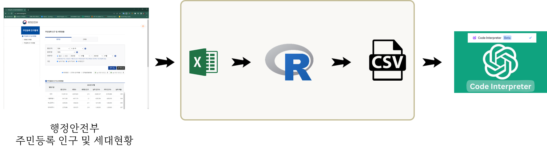
행정안전부 [주민등록 인구 및 세대현황](https://jumin.mois.go.kr/) 웹사이트에서 광명시 최근 데이터를 가져온다.
```{r}
library(tidyverse)
library(readxl)

raw_data <- read_excel("data/202307_202307_연령별인구현황_월간.xlsx", skip =3)

raw_data |>
  janitor::clean_names(ascii = FALSE) |>
  select(1:10) |>
  head() |>
  gt::gt()
```
## 가공데이터
```{r}
library(tidyverse)

pop_tbl <-
  read_rds("data/kwangmyung_pop.rds")

pop_tbl |>
  head() |>
  gt::gt()
```
## 챗GPT 데이터 변환
데이터를 가공한 후 챗GPT Code Interpreter 분석용으로 변환시켜 데이터를 전송한다.
```{r}
#| eval: false
pop_tbl |>
  write_csv("data/kwangmyung_pop.csv")
```
[[CSV 파일 다운로드](data/kwangmyung_pop.csv)]{.aside}
# 챗GPT Code Interpreter
::: {.panel-tabset}
### 데이터 불러오기
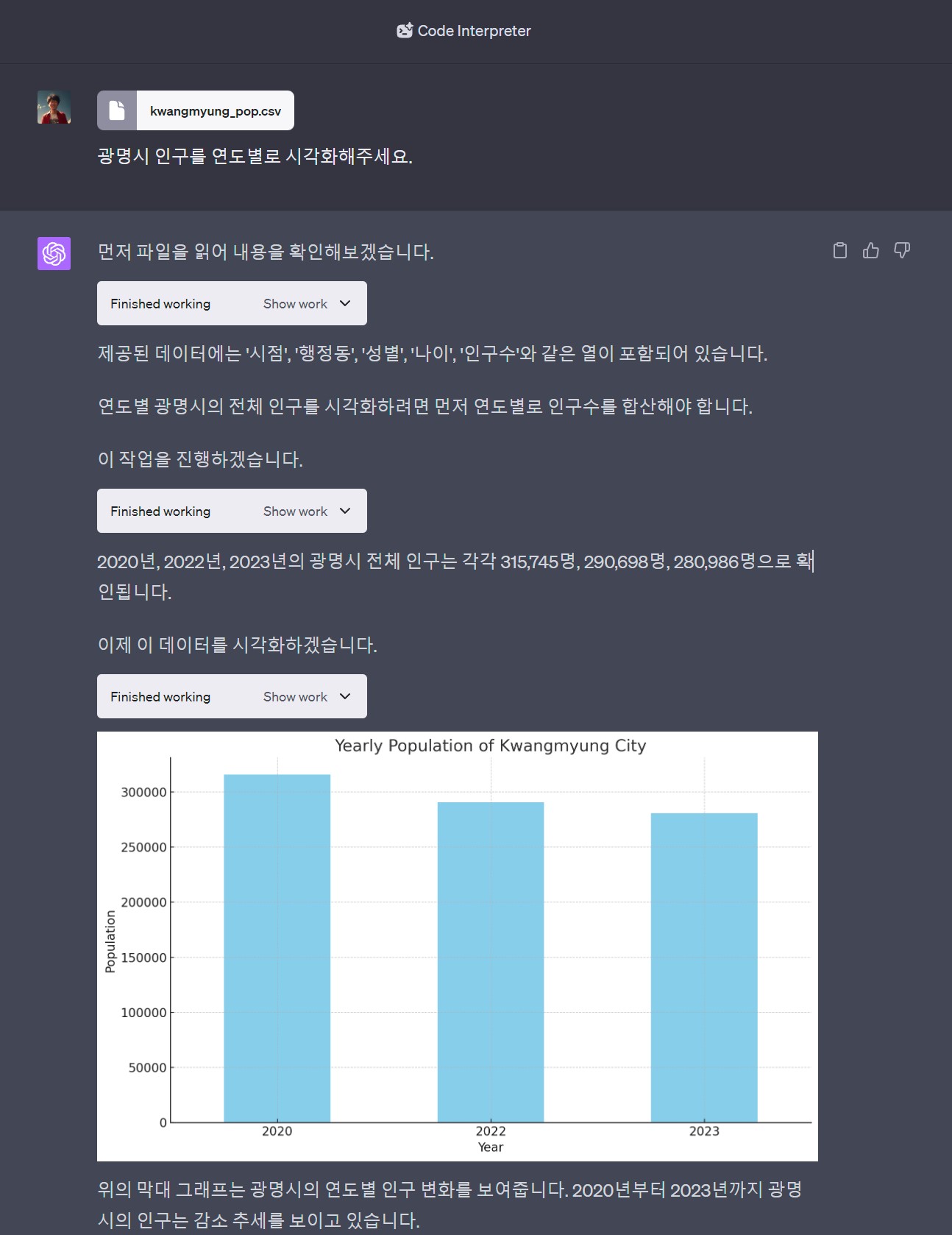
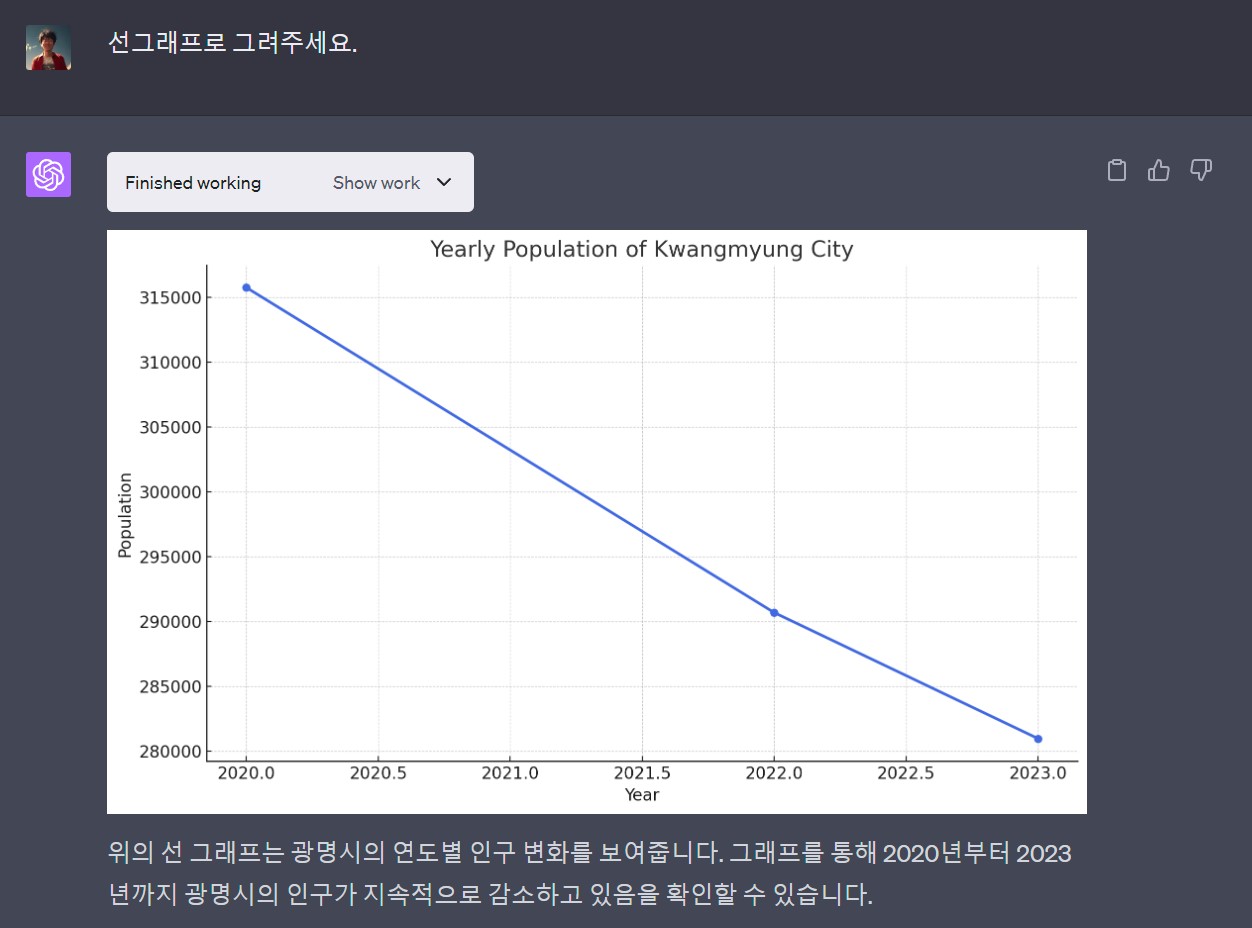
### 선그래프
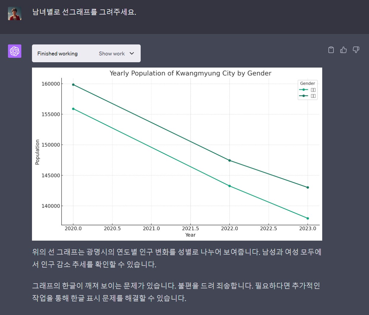
### 남녀별
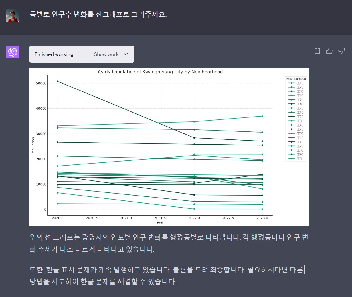
### 동별
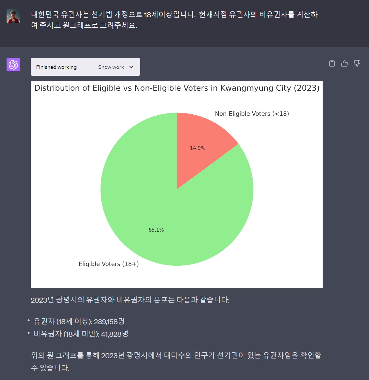
### 유권자 비율
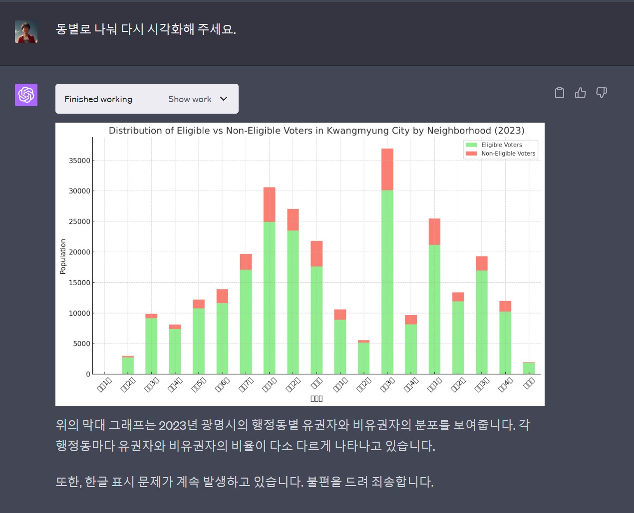
### 동별 유권자
### 동별 유권자(정렬)
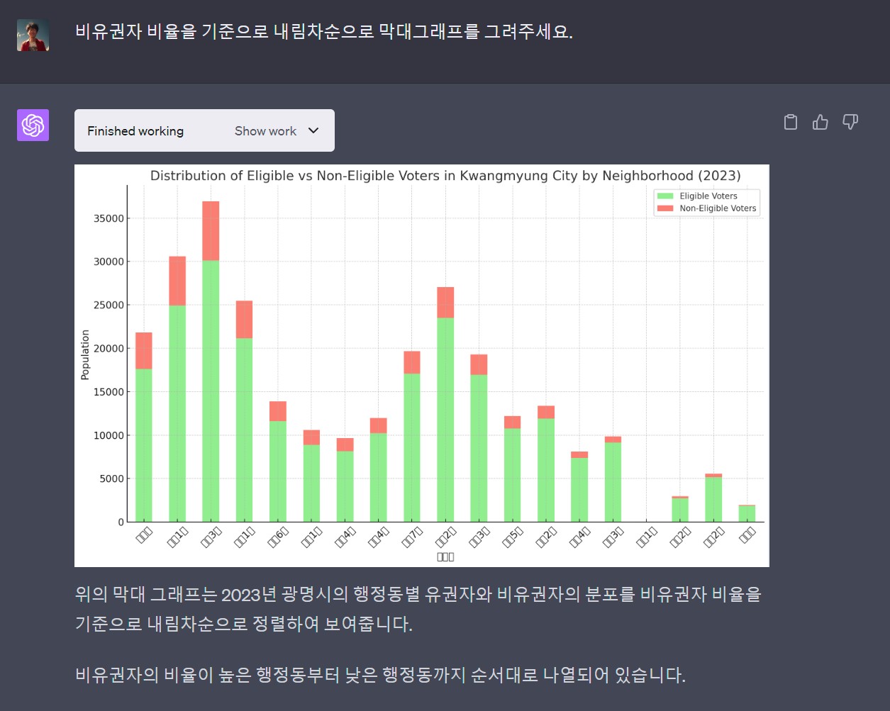
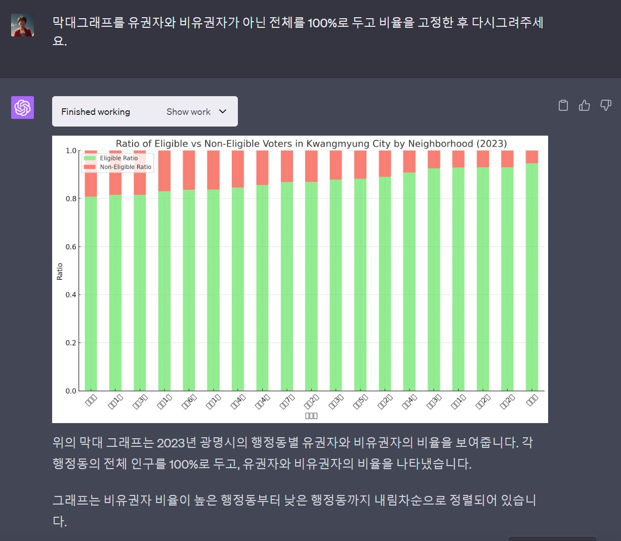
### 동별 유권자(비율)
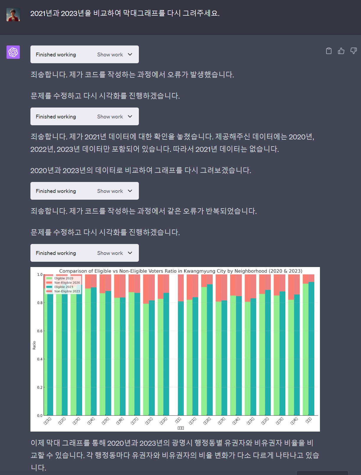
### 동별 유권자(비교)
### 노트북 내보내기
:::
[쥬피터 노트북 [다운로드](data/kwangmyung_population_analysis_v2.ipynb)]{.aside}
# 쥬피터 노트북 미리보기
{{< embed data/kwangmyung_population_analysis_v2.ipynb >}}
# 마무리 작업
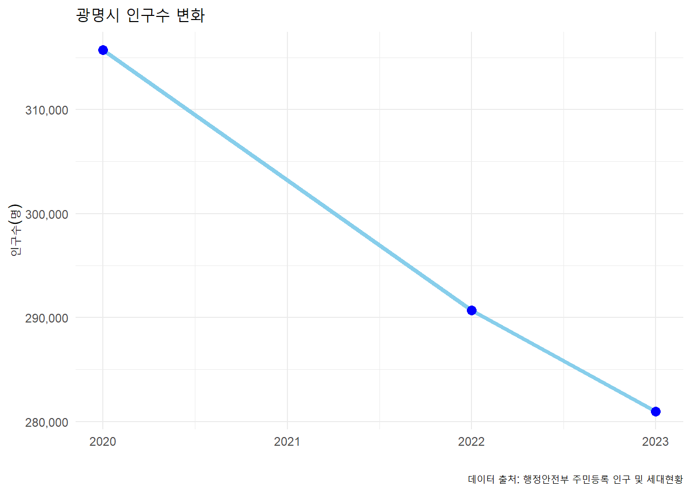
## 연도별 인구수
```{r}
library(tidyverse)

pop_tbl <-
  read_rds("data/kwangmyung_pop.rds")

pop_tbl |>
  mutate(시점 = ymd(시점)) |>
  mutate(연도 = year(시점)) |>
  group_by(연도) |>
  summarise(인구수 = sum(인구수)) |>
  ggplot(aes(x=연도, y=인구수)) +
    geom_line(color="skyblue", size=1.5) +
    geom_point(color="blue", size=3) +
    labs(title="광명시 인구수 변화", x="", y="인구수(명)",
         caption = "데이터 출처: 행정안전부 주민등록 인구 및 세대현황") +
    theme_minimal() +
    scale_y_continuous(labels = scales::comma)
```
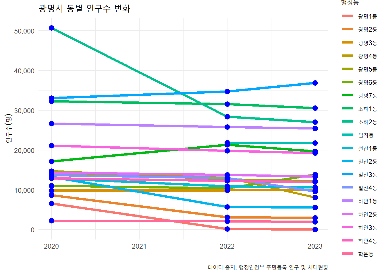
## 동별 인구수
```{r}
pop_tbl |>
  mutate(시점 = ymd(시점)) |>
  mutate(연도 = year(시점)) |>
  group_by(연도, 행정동) |>
  summarise(인구수 = sum(인구수)) |>
  ggplot(aes(x=연도, y=인구수, color = 행정동, group=행정동)) +
    geom_line(size=1.5) +
    geom_point(color="blue", size=3) +
    labs(title="광명시 동별 인구수 변화", x="", y="인구수(명)",
         caption = "데이터 출처: 행정안전부 주민등록 인구 및 세대현황") +
    theme_minimal() +
    scale_y_continuous(labels = scales::comma)
```
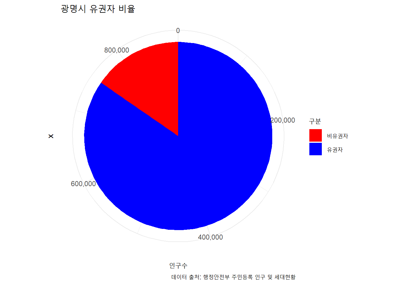
## 유권자 비율
```{r}
pop_tbl |>
  mutate(시점 = ymd(시점)) |>
  mutate(연도 = year(시점)) |>
  mutate(유권자 = ifelse(나이 >=18, "유권자", "비유권자"),
         유권자 = factor(유권자, levels = c("비유권자", '유권자'))) |>
  group_by(유권자) |>
  summarise(인구수 = sum(인구수)) |>
  ggplot(aes(x="", y=인구수, fill = 유권자)) +
    geom_bar(width = 1, stat = "identity") +
    coord_polar("y")  +
    labs(title="광명시 유권자 비율",
         caption = "데이터 출처: 행정안전부 주민등록 인구 및 세대현황",
         fill = "구분") +
    theme_minimal() +
    scale_y_continuous(labels = scales::comma) +
    scale_fill_manual(values = c(유권자 = "blue", 비유권자="red"))
```
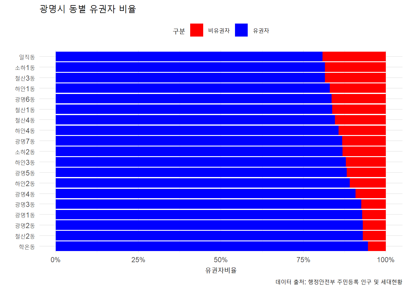
## 내림차순 유권자수
```{r}
pop_tbl |>
  mutate(시점 = ymd(시점)) |>
  mutate(연도 = year(시점)) |>
  filter(연도 == max(연도)) |>
  mutate(유권자 = ifelse(나이 >=18, "유권자", "비유권자"),
         유권자 = factor(유권자, levels = c("비유권자", '유권자'))) |>
  group_by(행정동, 유권자) |>
  summarise(인구수 = sum(인구수)) |>
  mutate(유권자비율 = 인구수/sum(인구수)) |>
  ungroup() |>

  # pivot_wider(names_from = 유권자, values_from = 인구수) |>
  # mutate(유권자비율 = 유권자/(비유권자+유권자)) |>
  # arrange(desc(유권자비율))

  # 시각화 -----------------
  ggplot(aes(x=fct_reorder2(행정동, 유권자, 유권자비율), y=유권자비율, fill = 유권자)) +
    geom_col() +
    coord_flip() +
    labs(title="광명시 동별 유권자 비율",
         caption = "데이터 출처: 행정안전부 주민등록 인구 및 세대현황",
         fill = "구분",
         x = "") +
    theme_minimal() +
    scale_y_continuous(labels = scales::percent) +
    scale_fill_manual(values = c(유권자 = "blue", 비유권자="red")) +
    theme(legend.position = "top")
```