---
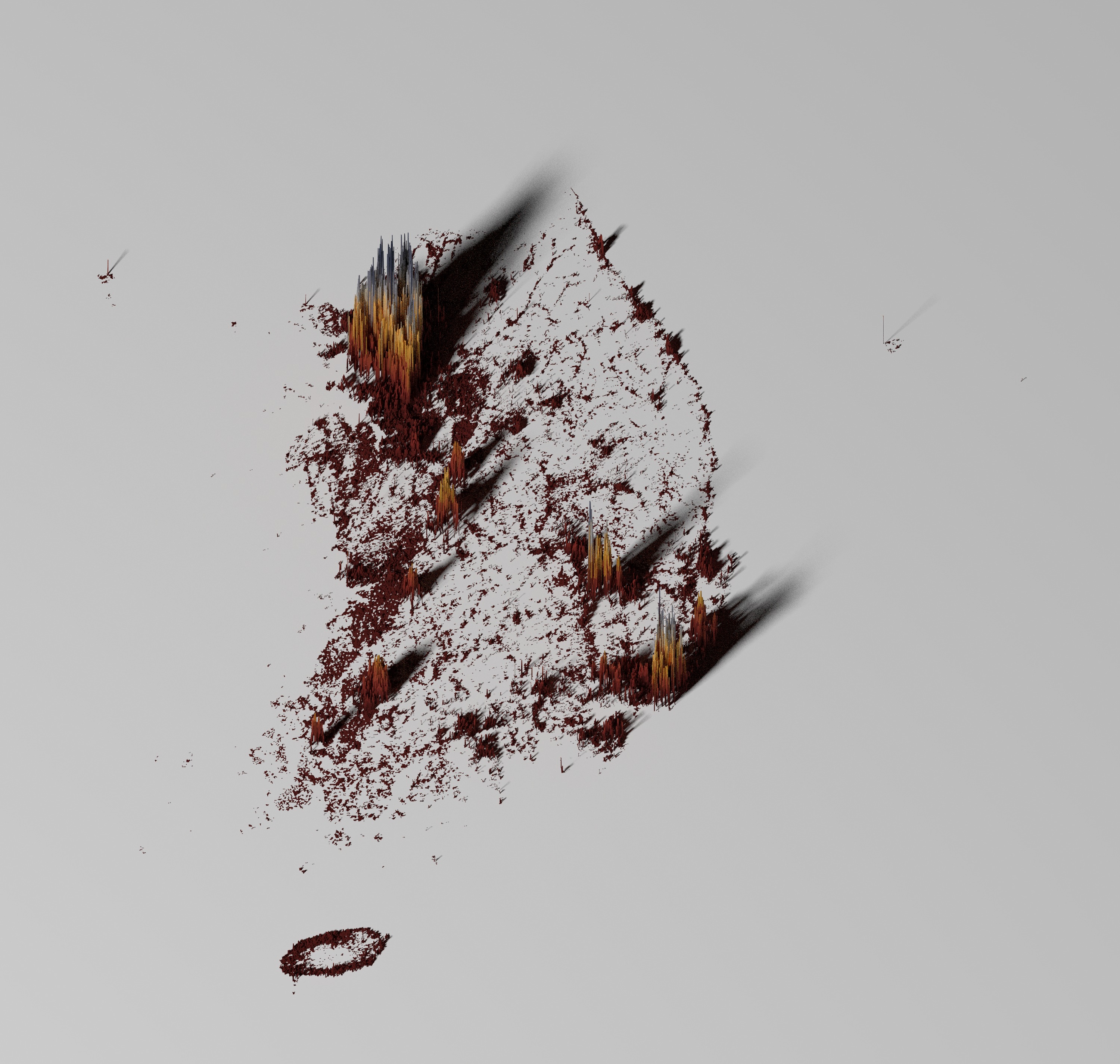
title: "스파이크(Spike map)"
subtitle: "3D 스파이크 지도"
description: |
3D 스파이크 지도를 제작해보자.
author:
- name: 이광춘
url: https://www.linkedin.com/in/kwangchunlee/
affiliation: 한국 R 사용자회
affiliation-url: https://github.com/bit2r
title-block-banner: true
format:
html:
theme: flatly
code-fold: true
code-overflow: wrap
toc: true
toc-depth: 3
toc-title: 목차
number-sections: true
highlight-style: github
self-contained: false
default-image-extension: jpg
filters:
- lightbox
lightbox: auto
bibliography: bibliography.bib
link-citations: true
csl: apa-single-spaced.csl
knitr:
opts_chunk:
message: false
warning: false
collapse: true
comment: "#>"
R.options:
knitr.graphics.auto_pdf: true
editor_options:
chunk_output_type: console
---
:::{.callout-tip}
### 소스코드
[Making crisp spike maps with R](https://github.com/milos-agathon/making-crisp-spike-maps-with-r)
:::
# 패키지
```{r}
### 0. PACKAGES
### ------------------------
libs <- c(
    "tidyverse", "R.utils",
    "httr", "sf", "stars",
    "rayshader"
)

# install missing libraries
installed_libs <- libs %in% rownames(installed.packages())
if (any(installed_libs == F)) {
    install.packages(libs[!installed_libs])
}

# load libraries
invisible(lapply(libs, library, character.only = T))
```
# 인구 데이터
인도주의적 영역에서 신뢰할 수 있는 인구 데이터를 확보하는 것은 생명을 구하는 활동의 우선순위를 정하는 데 매우 중요하다.
[KONTUR: Population Density Dataset](https://www.kontur.io/portfolio/population-dataset/) 인구 데이터 세트는 400m 해상도의 인구 수를 가진 H3 육각형으로 표현된다. 일반적인 정사각형 그리드 대신 H3 그리드를 사용하는 이유는 정사각형과 달리 육각형은 육각형 중심점과 인접한 셀의 중심 사이의 거리가 같기 때문이다. [Republic of Korea: Population Density for 400m H3 Hexagons](https://data.humdata.org/dataset/kontur-population-republic-of-korea) 데이터도 다운로드 가능하다.
```{r}
#| eval: false
#| label: spike-get-data
### 1. DOWNLOAD & UNZIP DATA
### ------------------------
url <-
    "https://geodata-eu-central-1-kontur-public.s3.amazonaws.com/kontur_datasets/kontur_population_KR_20220630.gpkg.gz"
file_name <- "korea-population.gpkg.gz"

get_population_data <- function() {
    res <- httr::GET(
        url,
        write_disk(file_name, overwrite = TRUE),
        progress()
    )

    R.utils::gunzip(file_name, remove = F)
}

get_population_data()
```
# 데이터 불러오기
```{r}
#| eval: false
#| label: spike-dataset
### 2. LOAD DATA
### -------------
load_file_name <- gsub(".gz", "", "korea-population.gpkg.gz")

crsWGS <- "+proj=tmerc +lat_0=38 +lon_0=128 +k=0.9999 +x_0=400000 +y_0=600000 +ellps=bessel +towgs84=-115.8,474.99,674.11,1.16,-2.31,-1.63,6.43 +units=m +no_defs"

get_population_data <- function() {
    pop_df <- sf::st_read(
        load_file_name
    ) |>
        sf::st_transform(crs = crsWGS)
}

pop_sf <- get_population_data()

head(pop_sf)
ggplot() +
    geom_sf(
        data = pop_sf,
        color = "grey10", fill = "grey10"
    )
```
# Shape to Raster
```{r}
#| eval: false
### 3. SHP TO RASTER
### ----------------

bb <- sf::st_bbox(pop_sf)

get_raster_size <- function() {
    height <- sf::st_distance(
        sf::st_point(c(bb[["xmin"]], bb[["ymin"]])),
        sf::st_point(c(bb[["xmin"]], bb[["ymax"]]))
    )
    width <- sf::st_distance(
        sf::st_point(c(bb[["xmin"]], bb[["ymin"]])),
        sf::st_point(c(bb[["xmax"]], bb[["ymin"]]))
    )

    if (height > width) {
        height_ratio <- 1
        width_ratio <- width / height
    } else {
        width_ratio <- 1
        height_ratio <- height / width
    }

    return(list(width_ratio, height_ratio))
}
width_ratio <- get_raster_size()[[1]]
height_ratio <- get_raster_size()[[2]]

size <- 3000
width <- round((size * width_ratio), 0)
height <- round((size * height_ratio), 0)

get_population_raster <- function() {
    pop_rast <- stars::st_rasterize(
        pop_sf |>
            dplyr::select(population, geom),
        nx = width, ny = height
    )

    return(pop_rast)
}

pop_rast <- get_population_raster()
plot(pop_rast)

pop_mat <- pop_rast |>
    as("Raster") |>
    rayshader::raster_to_matrix()

library(MetBrewer)
# Specify the palette name in its own variable so that
# we can reference it easily later.
pal <- "Demuth"
colors <- met.brewer(pal)

# cols <- rev(c(
#     '#00004d', '#342863', '#595078', '#7d7b8a', '#a7a88b'
# ))

texture <- grDevices::colorRampPalette(colors)(256)

# Create the initial 3D object
pop_mat |>
    rayshader::height_shade(texture = texture) |>
    rayshader::plot_3d(
        heightmap = pop_mat,
        solid = F,
        soliddepth = 0,
        zscale = 15,
        shadowdepth = 0,
        shadow_darkness = .95,
        windowsize = c(800, 800),
        phi = 65,
        zoom = .65,
        theta = -30,
        background = "white"
    )

# Use this to adjust the view after building the window object
rayshader::render_camera(phi = 75, zoom = .7, theta = 0)

library(rayrender)

rayshader::render_highquality(
    filename = "images/korea_population_2022.png",
    preview = FALSE,
    light = T,
    lightdirection = 225,
    lightaltitude = 60,
    lightintensity = 400,
    interactive = F,
    width = width, height = height
)
```