1 참고 웹사이트

2 원천 지도

국토교통부
- LX 한국국토정보공사, 구 한국지적공사
- 공간정보산업진흥원
  - VWorld, 공간정보오픈플랫폼
- 국토지리정보원
  - 국토정보플랫폼
  - 국가공간정보포털
    - 오픈마켓, 90m 표고 데이터: [국토지리정보원] 수치표고모델(DEM)_90M
대한민국 행정동 경계: admdongkor
대한민국 최신 행정구역(SHP) 다운로드

3 세계지도

출처: Fixing maps library data for Pacific centred (0°-360° longitude) display

코드

library(tidyverse)
library(sf)

# download.file(url = "https://gisco-services.ec.europa.eu/distribution/v2/countries/geojson/CNTR_RG_01M_2016_4326.geojson", destfile = "data/world.geojson", mode = "w")
# 
# world_sf <- giscoR::gisco_get_countries(
#   epsg = "4326",
#   region = "Asia",
#   resolution = "1",
#   cache = TRUE, 
#   update_cache = TRUE
# )

world_sf <- sf::st_read("data/world.geojson")
#> Reading layer `world' from data source `D:\tcs\map_challenge\data\world.geojson' using driver `GeoJSON'
#> Simple feature collection with 257 features and 6 fields
#> Geometry type: MULTIPOLYGON
#> Dimension:     XY
#> Bounding box:  xmin: -180 ymin: -89.9 xmax: 180 ymax: 83.66498
#> Geodetic CRS:  WGS 84

plot(st_geometry(world_sf))

코드

# 필요한 라이브러리를 불러옵니다.
library(ggplot2)
library(maps)

# 월드맵 데이터를 불러옵니다.
world_map <- map_data("world")

# ggplot2를 사용해 지도를 그립니다.
ggplot() +
  geom_polygon(data = world_map, aes(x = long, y = lat, group = group), fill = "white", color = "black") +
  coord_cartesian(xlim = c(-180, 180)) +
  theme_void()

코드

library(rnaturalearth)

# Get the world map data
world <- ne_countries(scale = "medium", returnclass = "sf")

# Shift the map to center on the Pacific Ocean
world_trans <- st_transform(st_wrap_dateline(world, options = c("WRAPDATELINE=YES", "DATELINEOFFSET=-180")), crs = "+proj=robin")

# Plot the world map
ggplot(data = world_trans) +
  geom_sf() +
  theme_minimal()

코드

asia_sf <- giscoR::gisco_get_countries(
  epsg = "4326",
  region = "Asia",
  resolution = "60",
  cache = TRUE,
  update_cache = TRUE
)

plot(st_geometry(asia_sf))

코드

library(tidyverse)
library(sf)
library(giscoR)

korea <- giscoR::gisco_get_countries(
    resolution = "1",
    country = "KOR"
) |>
    sf::st_transform("+proj=longlat +datum=WGS84 +no_defs +ellps=WGS84 +towgs84=0,0,0")

plot(st_geometry(korea))

코드

library(maps)

plot.map<- function(database,center,...){
    Obj <- map(database,...,plot=F)
    coord <- cbind(Obj[[1]],Obj[[2]])

    # split up the coordinates
    id <- rle(!is.na(coord[,1]))
    id <- matrix(c(1,cumsum(id$lengths)),ncol=2,byrow=T)
    polygons <- apply(id,1,function(i){coord[i[1]:i[2],]})

    # split up polygons that differ too much
    polygons <- lapply(polygons,function(x){
        x[,1] <- x[,1] + center
        x[,1] <- ifelse(x[,1]>180,x[,1]-360,x[,1])
        if(sum(diff(x[,1])>300,na.rm=T) >0){
          id <- x[,1] < 0
          x <- rbind(x[id,],c(NA,NA),x[!id,])
       }
       x
    })
    # reconstruct the object
    polygons <- do.call(rbind,polygons)
    Obj[[1]] <- polygons[,1]
    Obj[[2]] <- polygons[,2]

    map(Obj,...)
}

plot.map("world", center=210, col="white",bg="gray",
         fill=TRUE, ylim=c(-60,90),mar=c(0,0,0,0))

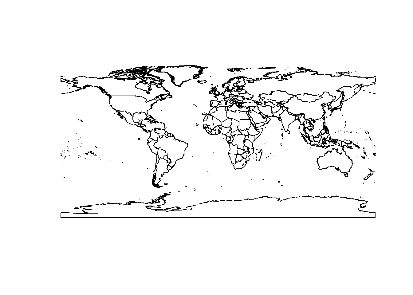
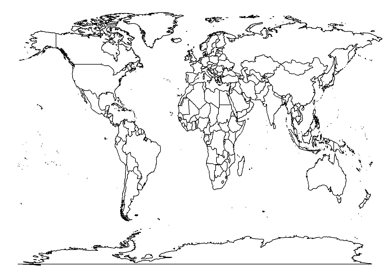
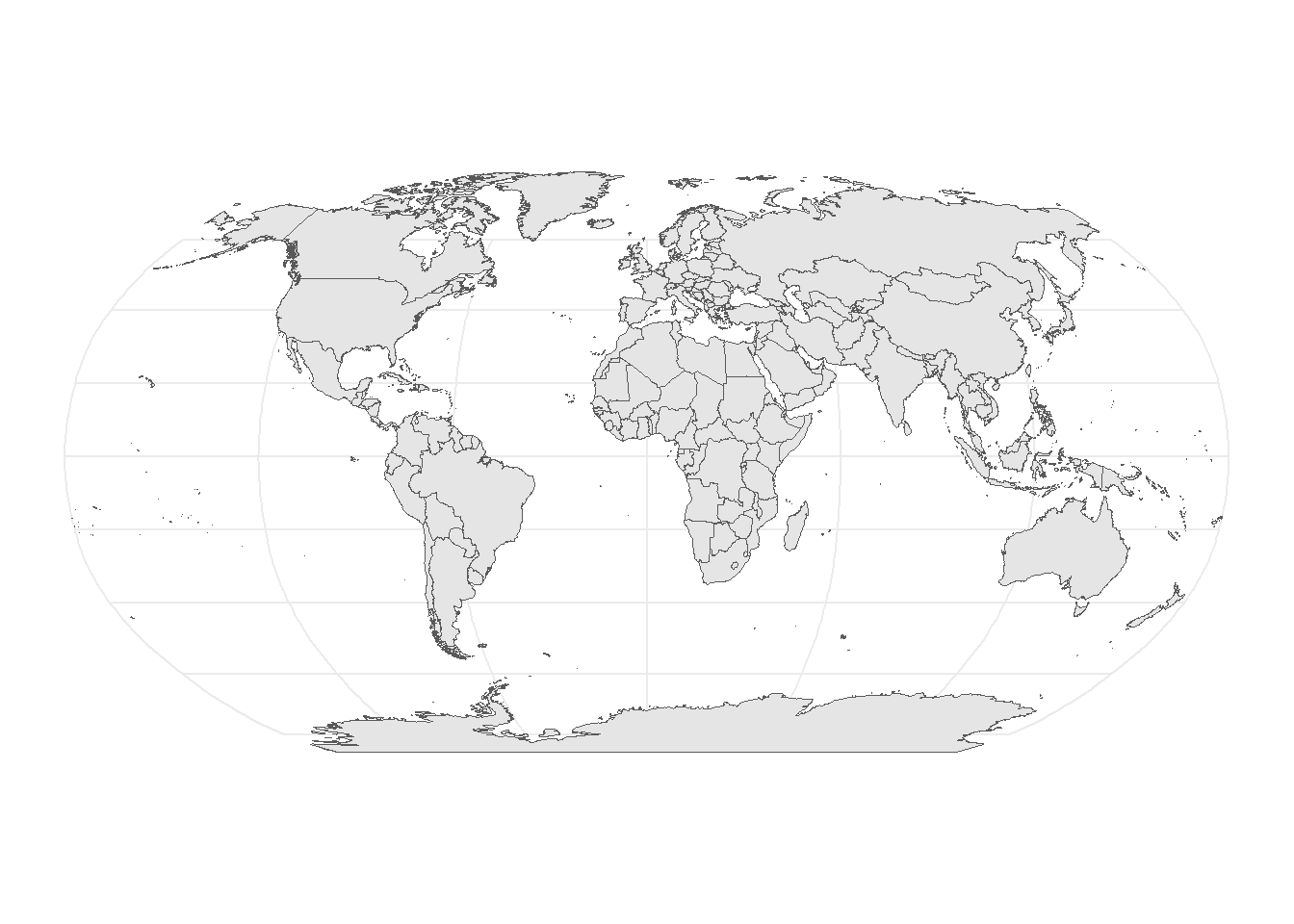
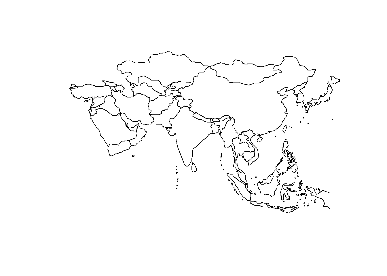
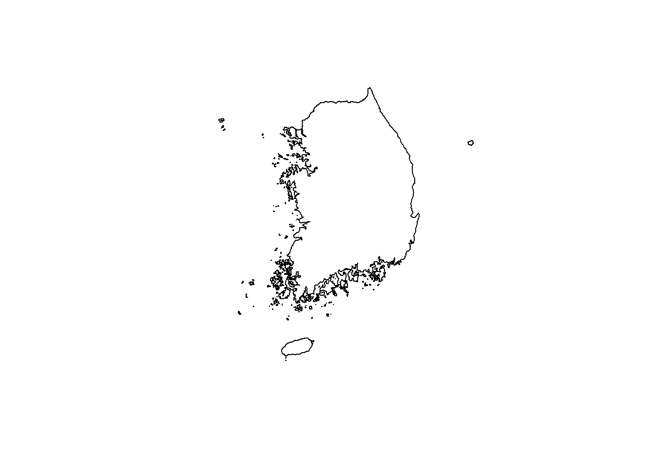
--- title: "지도제작 대회" subtitle: "챗GPT 지도제작을 위해서....." description: | 지도제작을 위한 다양한 정보를 모아 공개하고 있습니다. author: - name: 이광춘 url: https://www.linkedin.com/in/kwangchunlee/ affiliation: 한국 R 사용자회 affiliation-url: https://github.com/bit2r title-block-banner: true #title-block-banner: "#562457" format: html: theme: flatly code-fold: true code-overflow: wrap toc: true toc-depth: 3 toc-title: 목차 number-sections: true highlight-style: github self-contained: false filters: - lightbox lightbox: auto bibliography: bibliography.bib link-citations: true csl: apa-single-spaced.csl knitr: opts_chunk: message: false warning: false collapse: true comment: "#>" R.options: knitr.graphics.auto_pdf: true editor_options: chunk_output_type: console --- # 참고 웹사이트 - [#30DayMapChallenge 🌎🌏🌎](https://30daymapchallenge.com/) - [30 DAY MAP CHALLENGE IN R](https://david.frigge.nz/3RDayMapChallenge/) - [AbdoulMa/30DayMapChallenge](https://github.com/AbdoulMa/30DayMapChallenge) # 원천 지도 - [국토교통부](http://www.molit.go.kr/) - [LX 한국국토정보공사](https://www.lx.or.kr/), 구 한국지적공사 - [공간정보산업진흥원](http://www.spacen.or.kr/) - [VWorld, 공간정보오픈플랫폼](https://www.vworld.kr/) - [국토지리정보원](https://www.ngii.go.kr/) - [국토정보플랫폼](http://map.ngii.go.kr/) - [국가공간정보포털](https://www.nsdi.go.kr/) - 오픈마켓, 90m 표고 데이터: [국토지리정보원] 수치표고모델(DEM)_90M - [대한민국 행정동 경계: `admdongkor`](https://github.com/vuski/admdongkor) - [대한민국 최신 행정구역(SHP) 다운로드](http://www.gisdeveloper.co.kr/?p=2332) # 세계지도 [출처: [Fixing maps library data for Pacific centred (0°-360° longitude) display](https://stackoverflow.com/questions/5353184/fixing-maps-library-data-for-pacific-centred-0-360-longitude-display)]{.aside} :::{.panel-tabset} ### 세계지도: `giscoR` ```{r} library(tidyverse) library(sf) # download.file(url = "https://gisco-services.ec.europa.eu/distribution/v2/countries/geojson/CNTR_RG_01M_2016_4326.geojson", destfile = "data/world.geojson", mode = "w") # # world_sf <- giscoR::gisco_get_countries( # epsg = "4326", # region = "Asia", # resolution = "1", # cache = TRUE, # update_cache = TRUE # ) world_sf <- sf::st_read("data/world.geojson") plot(st_geometry(world_sf)) ``` ### 세계지도: `maps` ```{r} # 필요한 라이브러리를 불러옵니다. library(ggplot2) library(maps) # 월드맵 데이터를 불러옵니다. world_map <- map_data("world") # ggplot2를 사용해 지도를 그립니다. ggplot() + geom_polygon(data = world_map, aes(x = long, y = lat, group = group), fill = "white", color = "black") + coord_cartesian(xlim = c(-180, 180)) + theme_void() ``` ### 세계지도: `rnaturalearth` ```{r} library(rnaturalearth) # Get the world map data world <- ne_countries(scale = "medium", returnclass = "sf") # Shift the map to center on the Pacific Ocean world_trans <- st_transform(st_wrap_dateline(world, options = c("WRAPDATELINE=YES", "DATELINEOFFSET=-180")), crs = "+proj=robin") # Plot the world map ggplot(data = world_trans) + geom_sf() + theme_minimal() ``` ### 아시아 ```{r} asia_sf <- giscoR::gisco_get_countries( epsg = "4326", region = "Asia", resolution = "60", cache = TRUE, update_cache = TRUE ) plot(st_geometry(asia_sf)) ``` ### 대한민국 ```{r} library(tidyverse) library(sf) library(giscoR) korea <- giscoR::gisco_get_countries( resolution = "1", country = "KOR" ) |> sf::st_transform("+proj=longlat +datum=WGS84 +no_defs +ellps=WGS84 +towgs84=0,0,0") plot(st_geometry(korea)) ``` ### 태평양 중심 ```{r} #| eval: false library(maps) plot.map<- function(database,center,...){ Obj <- map(database,...,plot=F) coord <- cbind(Obj[[1]],Obj[[2]]) # split up the coordinates id <- rle(!is.na(coord[,1])) id <- matrix(c(1,cumsum(id$lengths)),ncol=2,byrow=T) polygons <- apply(id,1,function(i){coord[i[1]:i[2],]}) # split up polygons that differ too much polygons <- lapply(polygons,function(x){ x[,1] <- x[,1] + center x[,1] <- ifelse(x[,1]>180,x[,1]-360,x[,1]) if(sum(diff(x[,1])>300,na.rm=T) >0){ id <- x[,1] < 0 x <- rbind(x[id,],c(NA,NA),x[!id,]) } x }) # reconstruct the object polygons <- do.call(rbind,polygons) Obj[[1]] <- polygons[,1] Obj[[2]] <- polygons[,2] map(Obj,...) } plot.map("world", center=210, col="white",bg="gray", fill=TRUE, ylim=c(-60,90),mar=c(0,0,0,0)) ``` :::