지도제작 대회

소스코드

Create crisp topographic maps with R

1 패키지

코드

### 0. PACKAGES
### ------------------------
libs <- c(
    "elevatr", "terra", "tidyverse",
    "sf", "giscoR", "osmdata", "marmap"
)

# install missing libraries
installed_libs <- libs %in% rownames(installed.packages())
if (any(installed_libs == F)) {
    install.packages(libs[!installed_libs])
}

# load libraries
invisible(lapply(libs, library, character.only = T))

2 국가 데이터

코드

# 1. GET COUNTRY MAP
#------------------
crsLONGLAT <- "+proj=longlat +datum=WGS84 +no_defs"
get_country_sf <- function() {
    country_sf <- giscoR::gisco_get_countries(
        year = "2020",
        epsg = "4326",
        resolution = "10",
        country = "KR"
    ) |>
        sf::st_transform(crs = crsLONGLAT)

    return(country_sf)
}

country_sf <- get_country_sf()

3 국가 고도 데이터

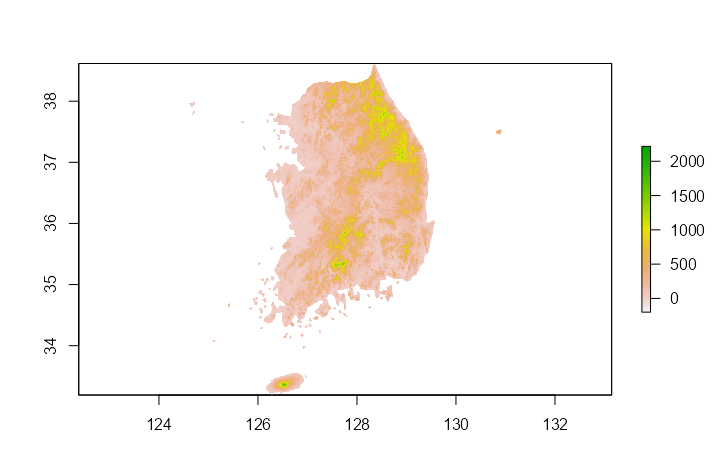
코드

# 2. GET COUNTRY ELEVATION DATA
#------------------------------
get_elevation_data <- function() {
    country_elevation <- elevatr::get_elev_raster(
        locations = country_sf,
        z = 7,
        clip = "locations"
    )

    return(country_elevation)
}

country_elevation <- get_elevation_data()
terra::plot(country_elevation)

4 BBOX 고도 데이터

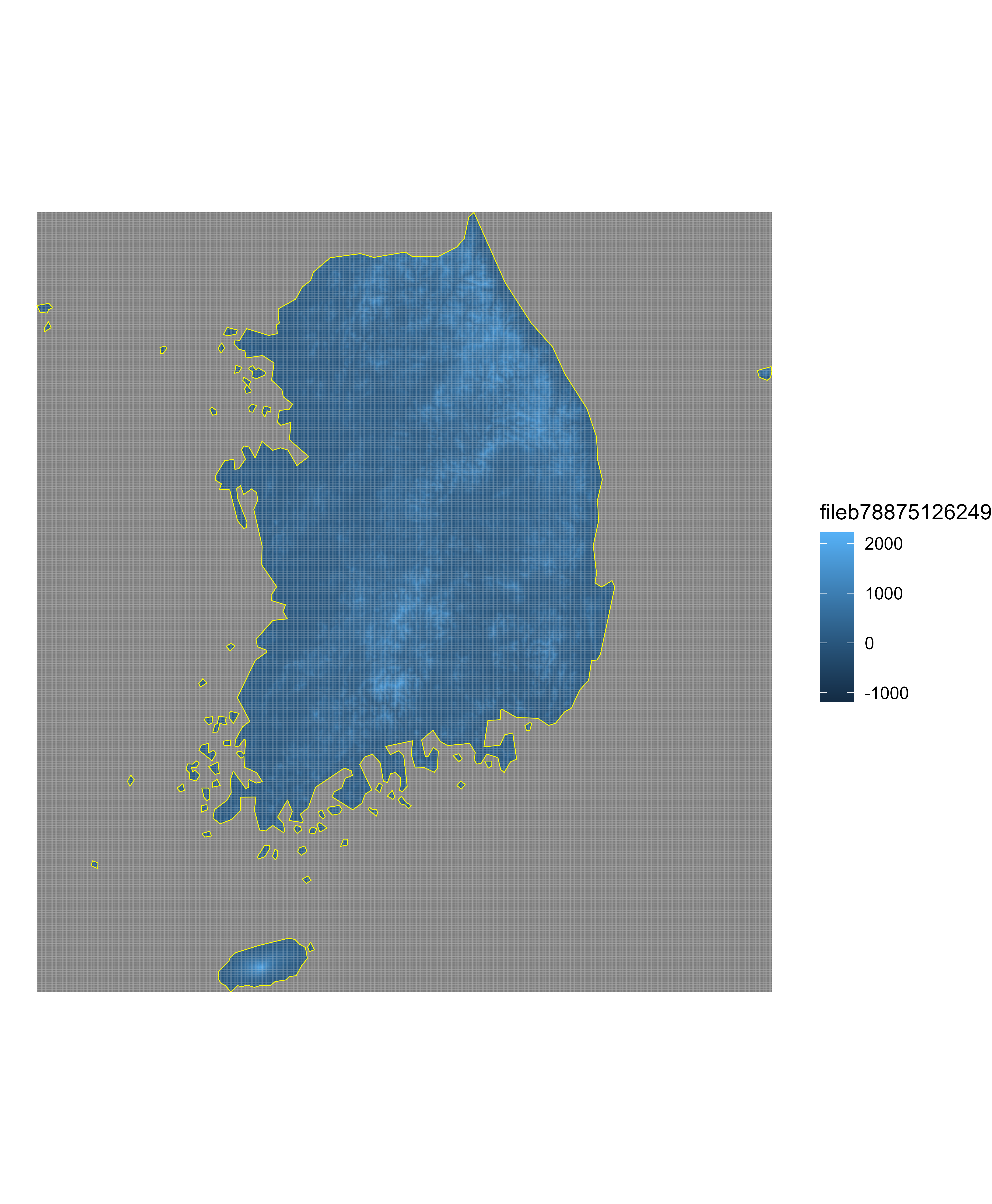
코드

# 3. GET BBOX ELEVATION DATA
#------------------------------
get_elevation_data_bbox <- function() {
    country_elevation <- elevatr::get_elev_raster(
        locations = country_sf,
        z = 7,
        clip = "bbox"
    )

    return(country_elevation)
}

country_elevation <- get_elevation_data_bbox() |>
    terra::rast()

코드

# 4. PLOT
#---------
kr_elevation_gg <- country_elevation |>
    as.data.frame(xy = TRUE) |> 
    ggplot() +
    geom_tile(
        aes(x = x, y = y, fill = fileb78875126249 )
    ) +
    geom_sf(
        data = country_sf,
        fill = "transparent", color = "yellow", size = .25
    ) +
    theme_void()

ggsave(
    filename = "images/kr_blue_map.png", width = 7, 
    height = 8.5, dpi = 600, device = "png", 
    kr_elevation_gg, bg = "white"
)

5 시각화

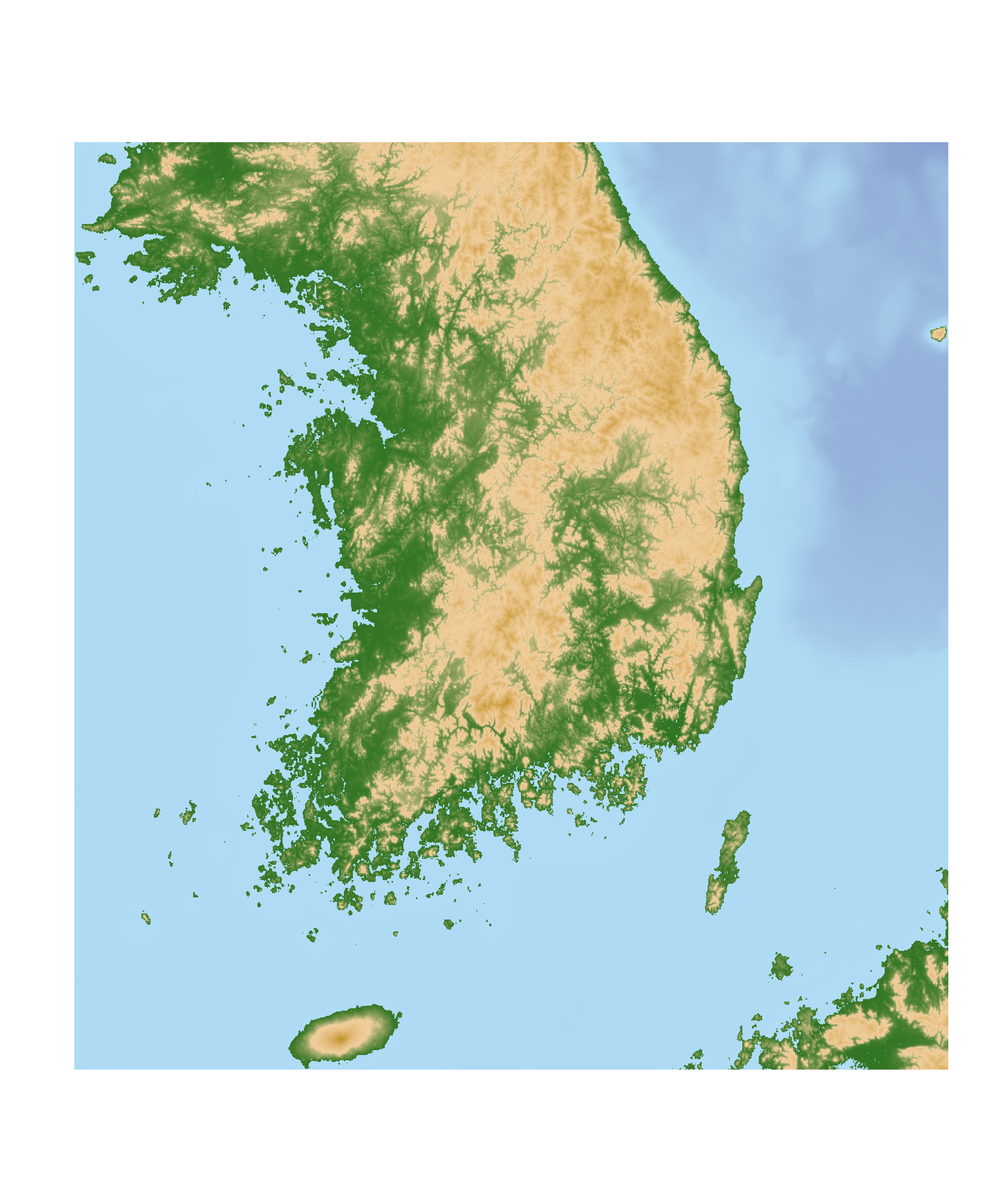
코드

# 7. FINAL MAP
#-------------

country_elevation_df <- country_elevation |>
    as.data.frame(xy = T) |>
    na.omit()

names(country_elevation_df)[3] <- "elevation"

country_map <-
    ggplot(data = country_elevation_df) +
    geom_raster(
        aes(x = x, y = y, fill = elevation),
        alpha = 1
    ) +
    marmap::scale_fill_etopo() +
    coord_sf(crs = crsLONGLAT) +
    labs(
        x = "",
        y = "",
        title = "",
        subtitle = "",
        caption = ""
    ) +
    theme_minimal() +
    theme(
        axis.line = element_blank(),
        axis.text.x = element_blank(),
        axis.text.y = element_blank(),
        axis.ticks = element_blank(),
        legend.position = "none",
        panel.grid.major = element_blank(),
        panel.grid.minor = element_blank(),
        plot.margin = unit(c(t = 0, r = 0, b = 0, l = 0), "cm"),
        plot.background = element_blank(),
        panel.background = element_blank(),
        panel.border = element_blank()
    )

country_map

ggsave(
    filename = "images/korea_topo_map.png", width = 7, 
    height = 8.5, dpi = 600, device = "png", 
    country_map, bg = "white"
)

6 추가작업

http://bboxfinder.com/ 에서 제거할 영역을 선정한다.

코드

# 5. CROP AREA
#--------------------
# 7.805786,38.779781,10.134888,41.294317
get_area_bbox <- function() {
    xmin <- 7.805786
    xmax <- 10.134888
    ymin <- 38.779781
    ymax <- 41.294317

    bbox <- sf::st_sfc(
        sf::st_polygon(list(cbind(
            c(xmin, xmax, xmax, xmin, xmin),
            c(ymin, ymin, ymax, ymax, ymin)
        ))),
        crs = crsLONGLAT
    )

    return(bbox)
}

bbox <- get_area_bbox()

crop_area_with_polygon <- function() {
    bbox_vect <- terra::vect(bbox)
    bbox_raster <- terra::crop(country_elevation, bbox_vect)
    bbox_raster_final <- terra::mask(
        bbox_raster, bbox_vect
    )
    return(bbox_raster_final)
}

bbox_raster_final <- crop_area_with_polygon()

bbox_raster_final |>
    as.data.frame(xy = T) |>
    ggplot() +
    geom_tile(
        aes(x = x, y = y, fill = file514862c13e19)
    ) +
    geom_sf(
        data = country_sf,
        fill = "transparent", color = "black", size = .25
    ) +
    theme_void()

# 6. GET REGION LINES
#--------------------
region <- "Sardinia"
# define longlat projection

sardinia_sf <- osmdata::getbb(
    region,
    format_out = "sf_polygon"
)

sardinia_sf

ggplot() +
    geom_sf(
        data = sardinia_sf$multipolygon,
        color = "red", fill = "grey80", size = .5
    ) +
    theme_void()

crop_region_with_polygon <- function() {
    region_vect <- terra::vect(sardinia_sf$multipolygon)
    region_raster <- terra::crop(country_elevation, region_vect)
    region_raster_final <- terra::mask(
        region_raster, region_vect
    )
    return(region_raster_final)
}

region_raster_final <- crop_region_with_polygon()

region_raster_final |>
    as.data.frame(xy = T) |>
    ggplot() +
    geom_tile(
        aes(x = x, y = y, fill = file514862c13e19)
    ) +
    geom_sf(
        data = country_sf,
        fill = "transparent", color = "black", size = .25
    ) +
    theme_void()