---
title: "지도제작 대회"
subtitle: "인구수 점(Point)"
description: |
인구수를 점으로 찍어보자.
author:
- name: 이광춘
url: https://www.linkedin.com/in/kwangchunlee/
affiliation: 한국 R 사용자회
affiliation-url: https://github.com/bit2r
title-block-banner: true
format:
html:
theme: flatly
code-fold: true
code-overflow: wrap
toc: true
toc-depth: 3
toc-title: 목차
number-sections: true
highlight-style: github
self-contained: false
default-image-extension: jpg
filters:
- lightbox
lightbox: auto
bibliography: bibliography.bib
link-citations: true
csl: apa-single-spaced.csl
knitr:
opts_chunk:
message: false
warning: false
collapse: true
comment: "#>"
R.options:
knitr.graphics.auto_pdf: true
editor_options:
chunk_output_type: console
---
:::{.callout-tip}
### 소스코드
[GIS 101: How do I map data points in R](https://github.com/milos-agathon/how-do-I-map-data-points-in-r)
:::
# `Geonames`
[Geonames - All Cities with a population > 1000](https://data.opendatasoft.com/explore/dataset/geonames-all-cities-with-a-population-1000%40public) 데이터셋은 API 혹은 `.xlsx`, `.csv` 파일로 다운로드 받아 사용이 가능하다.
```{r}
#| eval: false
library(httr)

geonames <- GET("https://data.opendatasoft.com/api/records/1.0/search/?dataset=geonames-all-cities-with-a-population-1000%40public&q=&sort=name&facet=feature_code&facet=cou_name_en&facet=timezone&timezone=Asia%2FSeoul")

geonames_tbl <- jsonlite::fromJSON(content(geonames, "text"))

geonames_tbl$records
```
## 인구수
```{r}
library(readxl)
library(tidyverse)
geonames_raw <- read_excel("data/geonames-all-cities-with-a-population-1000@public.xlsx") %>%
janitor::clean_names()
korea_raw <- geonames_raw %>%
select(name, country_code, population, coordinates) %>%
filter(country_code == "KR") %>%
separate(coordinates, into = c("lat", "long"), sep = ",", convert = TRUE)
korea <- korea_raw %>%
mutate(도시명 = c("한천리", "청송군", "청산", "함열", "동면",
"유려", "심원", "법성", "연천", "동복", "산티옥",
"난겐", "제주시", "안남", "금정", "상사", "승주",
"불갑", "원주", "벌교", "법원", "광주", "신안",
"군서", "군북", "신동", "조성", "문경", "임실",
"용산동", "하성", "겸백", "영광", "예산",
"양주", "당진", "상주", "고창", "해남", "주문진",
"청주시", "진천", "가이게투리", "규암", "선원",
"탄현", "울산", "의정부시", "상주", "문경", "가평",
"현풍", "홍성", "정옥", "장성", "신현",
"광명", "회남", "용산", "번암", "월곶", "장흥",
"아이센", "영덕", "전산", "부여", "부산", "오산",
"고성", "경산시", "군위", "장흥", "성남시",
"미조", "옥곡", "대구", "김제", "김천", "익산",
"광양", "통해", "동이", "오남", "봉강", "용화",
"성환", "강포", "싱왕", "정읍", "강동", "청풍",
"진상", "옹룡", "봉래", "인계", "비인", "공주",
"충주", "안양시", "장평", "해안", "문덕",
"미력", "해리", "물량", "구림", "대전", "고성",
"교사이", "연무", "화남", "서상", "서석", "남면",
"해령", "송광", "상하", "동계", "서울", "아산",
"괴산", "하양", "진안군", "장안", "남양주", "안내",
"교동", "진월", "주암", "대산", "영동", "백전",
"토성", "공음", "담양", "보령", "속초", "광주",
"구룡포", "강화군", "청양", "진주", "진잠", "안산시",
"발금", "별량", "남면", "태백", "푸안", "화순", "화천", "전주",
"지도", "이원", "화원", "서귀포", "병곡", "통진",
"진접", "보성", "영암", "염산", "칠보", "아이센",
"포항", "목포", "구미", "김해", "천안", "일광",
"산서", "산내", "덕진", "대마", "완주", "수원",
"평창", "군포", "인천", "화성시", "창원", "창수",
"홍농", "양사", "광탄", "유치", "연일", "양평",
"왜관", "심천", "무안", "강릉", "화도", "와부",
"설천", "대합", "동래", "네이츠", "신탄신", "금산",
"추풍령", "안동", "청남", "황간", "창녕", "여주",
"밀양", "홍천", "철원", "한남", "세종", "반남",
"금성", "하동", "영천", "춘천", "백수", "성수",
"학산", "순천", "군산", "청평", "송강동", "수동",
"외서", "낙월", "강진", "용안", "동래", "나주",
"문산", "구리시", "창평", "하점", "압해", "도포",
"군서", "흥해", "유성", "이양", "태산리", "부천시",
"논산", "광양", "이천시", "여수", "웅상", "내선",
"파주", "청성", "서산", "경주", "관촌", "상월", "시종",
"구정", "동면", "마산", "고양시", "기장", "안성",
"청하", "군북", "송해", "광적", "관인", "방산",
"노동", "나산", "임자", "양구", "일로", "오천",
"신서", "부평", "화양", "세지", "해보", "군남",
"쌍치", "양산", "옥천", "구례", "푸발", "삼승",
"삼산", "신안", "정량", "해제")) %>%
filter(population > 0) %>%
arrange(desc(population))
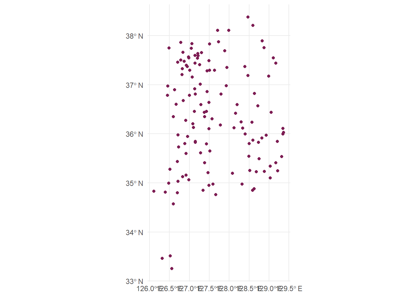
korea
```
# 지도
## DF → `sf` 객체
```{r}
crsLONGLAT <- "+proj=longlat +datum=WGS84 +no_defs +ellps=WGS84 +towgs84=0,0,0"

korea_sf <- korea |>
    sf::st_as_sf(
        coords = c("long", "lat"),
        crs = crsLONGLAT
    )

ggplot() +
    geom_sf(
        data = korea_sf,
        color = "#7d1d53", fill = "#7d1d53"
    )
```
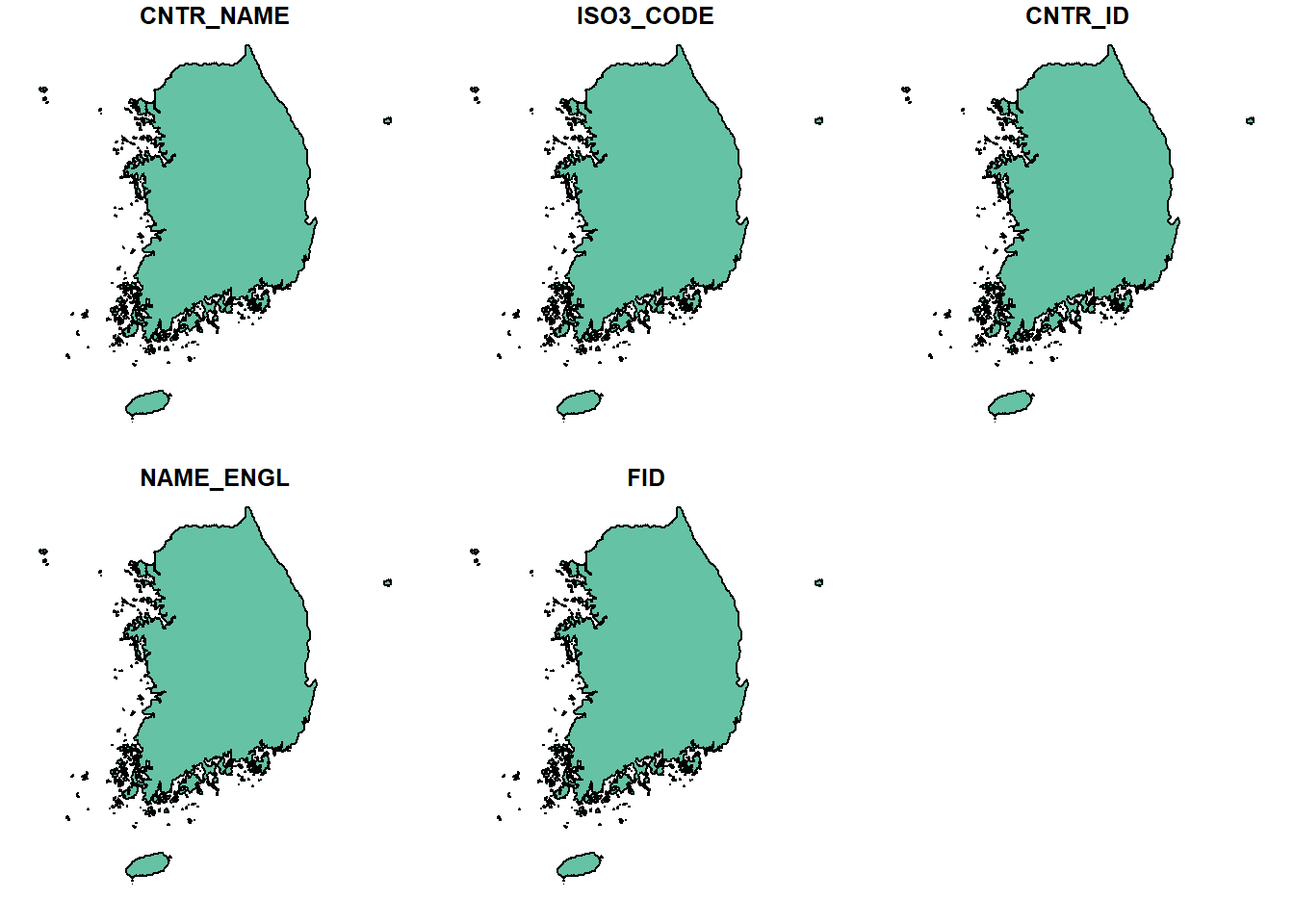
## `shapefile`
[`giscoR`](https://ropengov.github.io/giscoR/) 유로스탯 - GISCO(유럽집행위원회 지리정보시스템)에서 데이터를 다운로드 없이 바로 사용할 수 있는 가벼운 API를 제공한다.
```{r}
kr <- giscoR::gisco_get_countries(
    resolution = "1",
    country = "KOR") |>
    sf::st_transform(crsLONGLAT)

plot(kr)
```
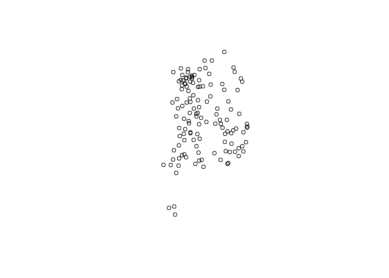
## 결합
```{r}
kr_pop_sf <- sf::st_intersection(korea_sf, kr)

plot(sf::st_geometry(kr_pop_sf))
```
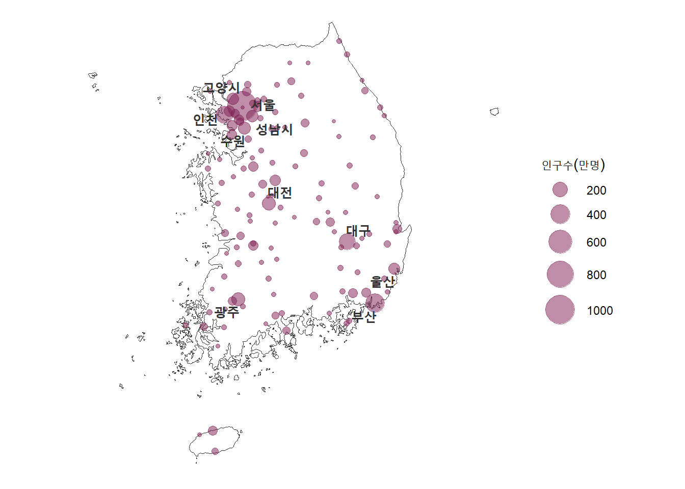
# 시각화
인구수가 높은 도시 10개를 뽑아 시각화해보자.
```{r}
extrafont::loadfonts("win")

korea_sf <- korea_sf %>%
  mutate(population = population / 10^4)

korea_city <- korea_sf %>%
    mutate(long = unlist(purrr::map(geometry, 1)),
           lat = unlist(purrr::map(geometry,2))) %>%
    dplyr::select(
        도시명, long, lat, population) |>
    sf::st_drop_geometry() |>
    as.data.frame() |>
    dplyr::arrange(desc(population))

ggplot() +
    geom_sf(
        data = kr,
        color = "grey20", fill = "transparent"
    ) +
    geom_sf(
        data = korea_sf,
        aes(size = population),
        color = "#7d1d53", fill = "#7d1d53",
        alpha = .5
    ) +
    scale_size(
        range = c(1, 10),
        breaks = scales::pretty_breaks(n=6)
    )  +
    theme_minimal(base_family = "MaruBuri") +
        theme(
            axis.line = element_blank(),
            axis.text.x = element_blank(),
            axis.text.y = element_blank(),
            axis.ticks = element_blank(),
            axis.title.x = element_blank(),
            axis.title.y = element_blank(),
            panel.grid.major = element_blank(),
            panel.grid.minor = element_blank(),
            plot.margin = unit(
                c(t = 0, r = 0, b = 0, l = 0), "lines"
            ),
            plot.background = element_rect(fill = "white", color = NA),
            panel.background = element_rect(fill = "white", color = NA),
            legend.background = element_rect(fill = "white", color = NA),
            panel.border = element_blank(),
      ) +
    ggrepel::geom_text_repel(korea_city %>% slice(1:10),
        mapping = aes(x = long, y = lat, label = 도시명),
        colour = "grey20",
        fontface = "bold",
        size = 4,
        family = "MaruBuri"
    )   +
    labs(size="인구수(만명)")
```