5 . 분포 / distribution
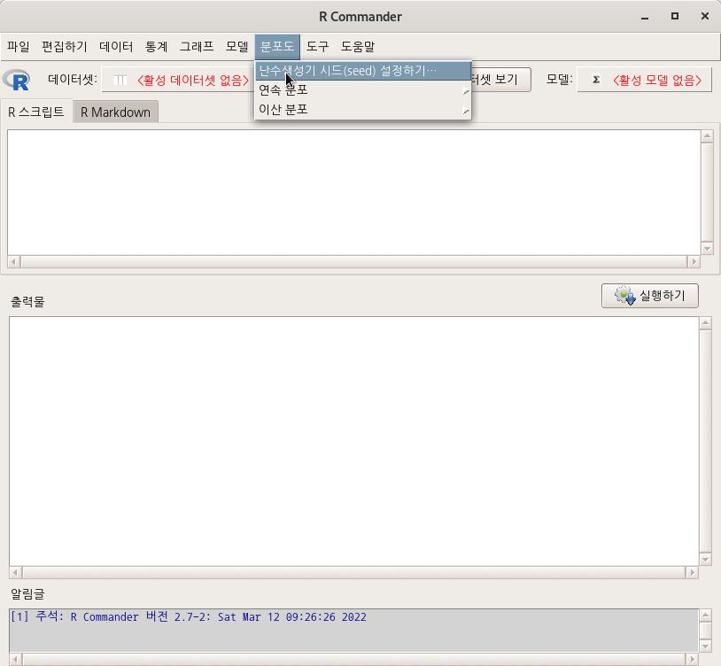
5.1 난수생성기 시드(seed) 생성기… / Distributions > Set random number generator seed…
Linux 사례 (MX 21)
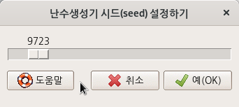
번호 하나를 선택한다. 그 번호는 앞으로 생성되는 난수 값들을 기억한다.
Linux 사례 (MX 21)
set.seed(9723)5.2 분포도
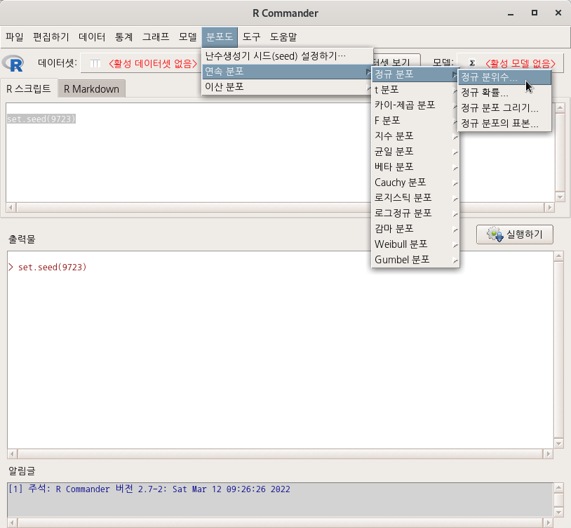
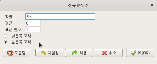
5.2.1 연속 분포 > 정규 분포 > 정규 분위수…/ Distributions > Continuous distributions > Normal distribution > Normal quantiles…
Linux 사례 (MX 21)
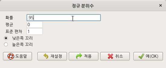
확률을 넣고, 분포도의 (꼬리) 방향을 정해주면, 분위수가 계산된다. 을 95%(.095)로 선택해보자. 선택에 따라 어떻게 값이 변하는지 살펴보자.
Linux 사례 (MX 21)
Linux 사례 (MX 21)
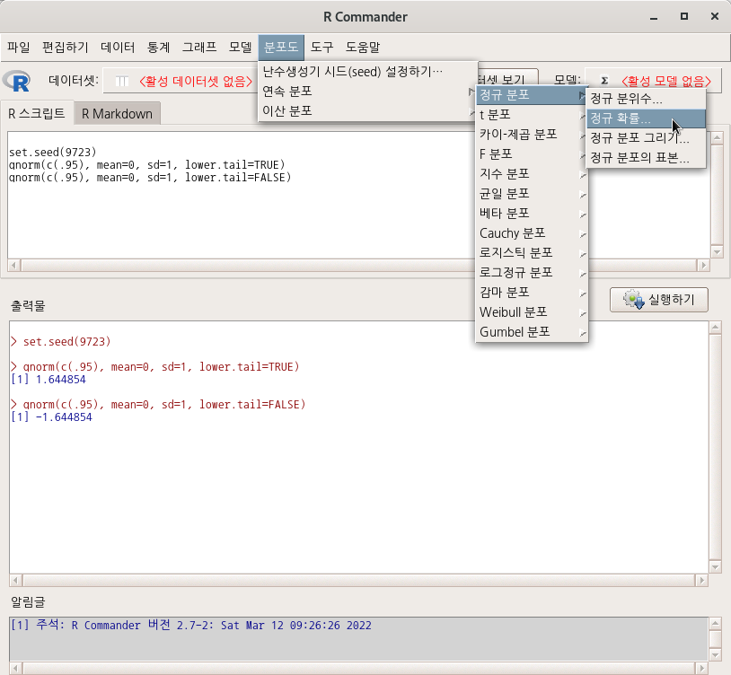
## [1] 1.644854## [1] -1.644854아래 화면에서 95% 확률로 방향의 값을 확인할 수 있다.

Linux 사례 (MX 21)
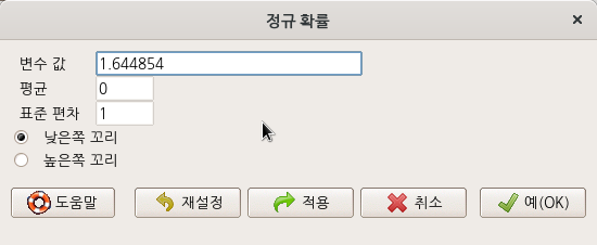
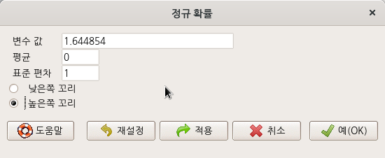
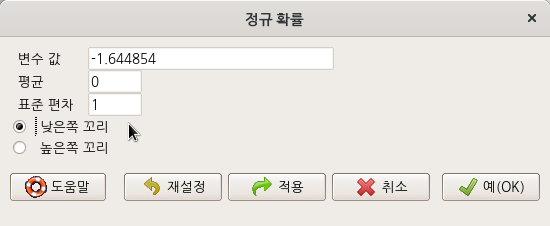
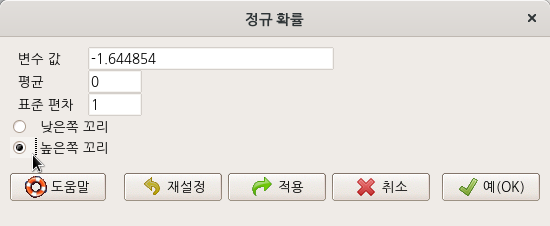
5.2.2 연속 분포 > 정규 분포 > 정규 확률…/ Distributions > Continuous distributions > Normal distribution > Normal probabilities…
Linux 사례 (MX 21)
사례 값을 넣고, 분포도의 (꼬리) 방향을 정해주면 확률이 계산된다.
Linux 사례 (MX 21)
Linux 사례 (MX 21)
Linux 사례 (MX 21)
Linux 사례 (MX 21)
## [1] 0.95## [1] 0.04999996## [1] 0.04999996## [1] 0.95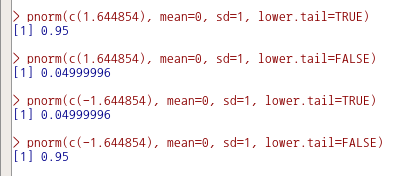
Linux 사례 (MX 21)
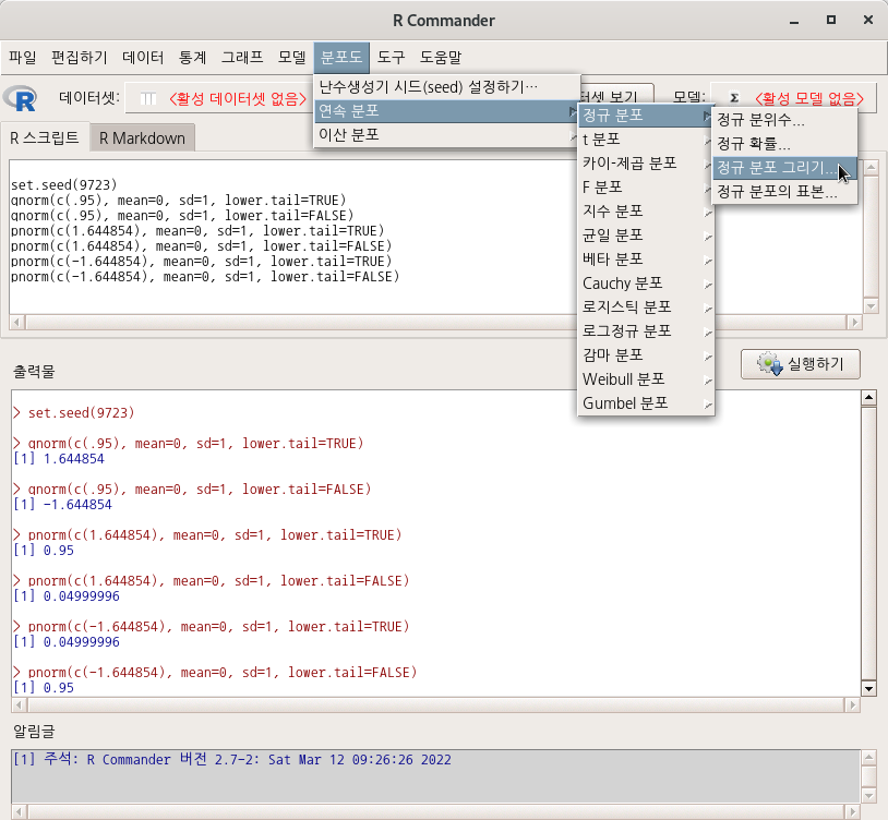
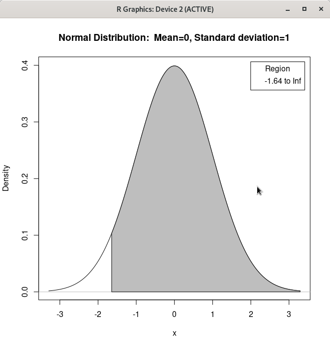
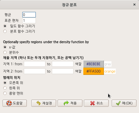
5.2.3 연속 분포 > 정규 분포 > 정규 분포 그리기… / Distributions > Continuous distributions > Normal distribution > Plot normal distribution…
Linux 사례 (MX 21)
<밀도 함수 그리기 (Plot density function)>를 선택하고

Linux 사례 (MX 21)
local({
  .x <- seq(-3.291, 3.291, length.out=1000)
  plotDistr(.x, dnorm(.x, mean=0, sd=1), cdf=FALSE, xlab="x", ylab="Density",
  main=paste("Normal Distribution:  Mean=0, Standard deviation=1"), regions=list(c(-1.644854, Inf)),
  col=c('#BEBEBE', '#FFA500'), legend.pos='topright')
})
Linux 사례 (MX 21)
Linux 사례 (MX 21)
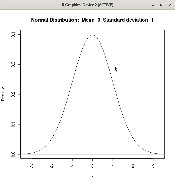
local({
  .x <- seq(-3.291, 3.291, length.out=1000)
  plotDistr(.x, dnorm(.x, mean=0, sd=1), cdf=FALSE, xlab="x", ylab="Density",
  main=paste("Normal Distribution:  Mean=0, Standard deviation=1"))
})
Linux 사례 (MX 21)
Linux 사례 (MX 21)
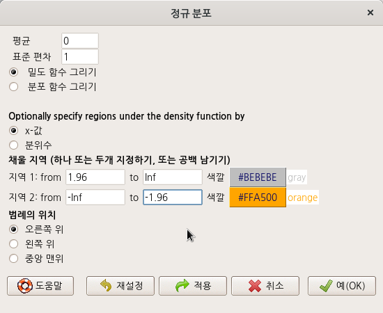
local({
.x <- seq(-3.291, 3.291, length.out=1000)
plotDistr(.x, dnorm(.x, mean=0, sd=1), cdf=FALSE, xlab="x", ylab="Density",
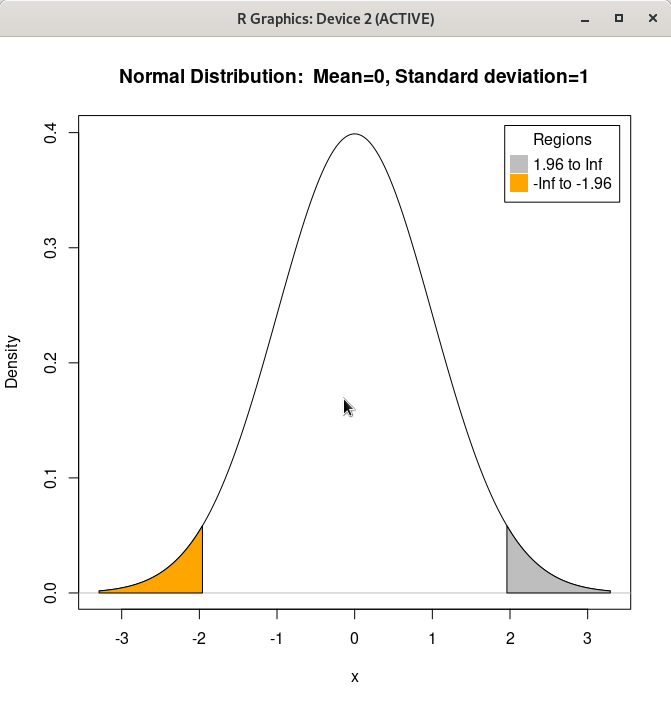
main=paste("Normal Distribution: Mean=0, Standard deviation=1"), regions=list(c(1.96, Inf), c(-Inf,
-1.96)), col=c('#BEBEBE', '#FFA500'), legend.pos='topright')
})
Linux 사례 (MX 21)
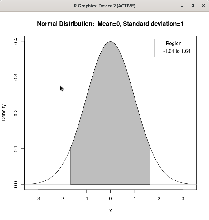
<밀도 함수 그리기 (Plot density function)>를 선택하고 를 선택한 상황에서 몇 몇 사례를 만들어본다.
Linux 사례 (MX 21)
에 입력할 수 있는 범위는 0에서 1까지의 확률이다. 이 범위 안에 들어오는 숫자는 아래 명령문 내부 regions에서 보이듯이 분위수로 전환된다.
local({
  .x <- seq(-3.291, 3.291, length.out=1000)
  plotDistr(.x, dnorm(.x, mean=0, sd=1), cdf=FALSE, xlab="x", ylab="Density",
  main=paste("Normal Distribution:  Mean=0, Standard deviation=1"), regions=list(c(-1.64485362695147,
  1.64485362695147)), col=c('#BEBEBE', '#FFA500'), legend.pos='topright')
})
Linux 사례 (MX 21)

Linux 사례 (MX 21)
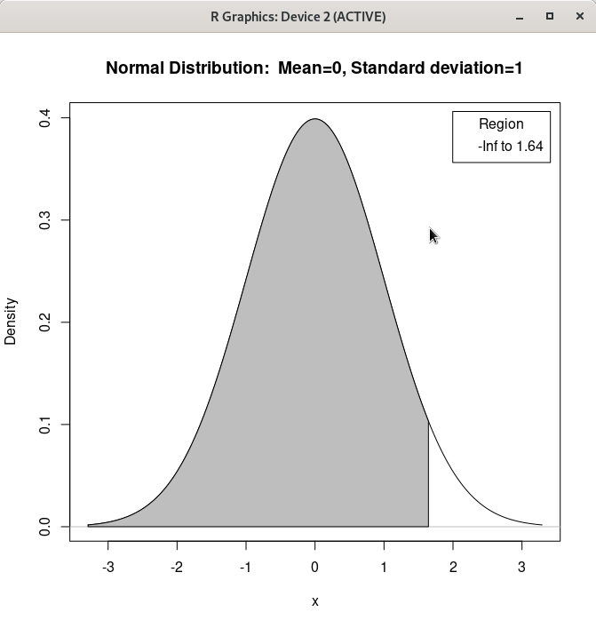
local({
  .x <- seq(-3.291, 3.291, length.out=1000)
  plotDistr(.x, dnorm(.x, mean=0, sd=1), cdf=FALSE, xlab="x", ylab="Density",
  main=paste("Normal Distribution:  Mean=0, Standard deviation=1"), regions=list(c(-Inf,
  1.64485362695147)), col=c('#BEBEBE', '#FFA500'), legend.pos='topright')
})
Linux 사례 (MX 21)

Linux 사례 (MX 21)
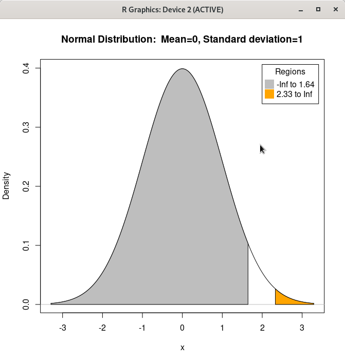
local({
  .x <- seq(-3.291, 3.291, length.out=1000)
  plotDistr(.x, dnorm(.x, mean=0, sd=1), cdf=FALSE, xlab="x", ylab="Density",
  main=paste("Normal Distribution:  Mean=0, Standard deviation=1"), regions=list(c(-Inf,
  1.64485362695147), c(2.32634787404084, Inf)), col=c('#BEBEBE', '#FFA500'), legend.pos='topright')
})
Linux 사례 (MX 21)
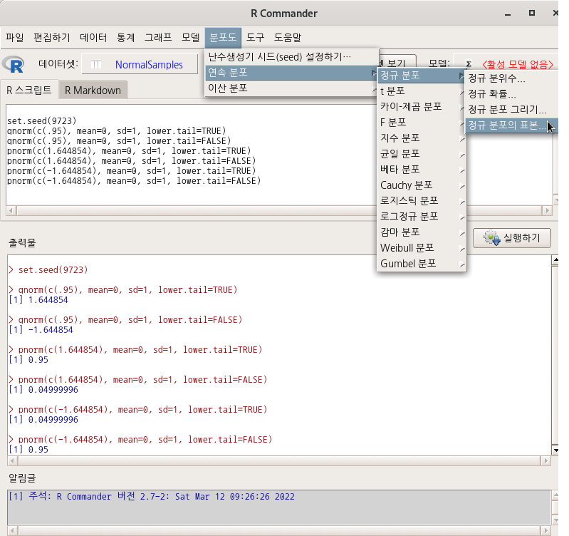
5.2.4 연속 분포 > 정규 분포 > 정규 분포의 표본…/ Distributions > Continuous distributions > Normal distributions > Sample from normal distribution…
Linux 사례 (MX 21)
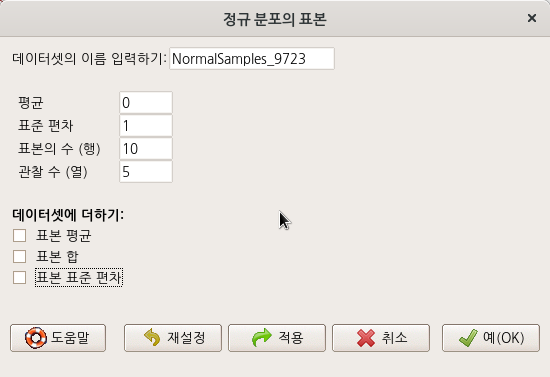
창에는 다양한 선택 기능이 있다. 표본의 수 (행)과 관찰 수 (열)에 표본 범위를 넣자. ’데이터셋의 이름 입력하기’에는 원하는 이름을 넣을 수 있다. 나는 set.seed(번호)를 연상시키는 번호를 입력하기도 한다.
Linux 사례 (MX 21)
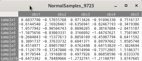
set.seed(9723)
NormalSamples_9723 <- as.data.frame(matrix(rnorm(10*5, mean=0, sd=1), ncol=5))
rownames(NormalSamples_9723) <- paste("sample", 1:10, sep="")
colnames(NormalSamples_9723) <- paste("obs", 1:5, sep="")
Set random number generator seed… 참고
Linux 사례 (MX 21)