영어작문 성적

library(bitData)
#> Warning: replacing previous import 'jsonlite::flatten' by 'purrr::flatten' when
#> loading 'bitData'
#> 
#> Attaching package: 'bitData'
#> The following object is masked from 'package:datasets':
#> 
#>     co2
library(tidyverse)
#> ── Attaching packages ─────────────────────────────────────── tidyverse 1.3.1 ──
#> ✔ ggplot2 3.3.6      ✔ purrr   0.3.4 
#> ✔ tibble  3.1.8      ✔ dplyr   1.0.10
#> ✔ tidyr   1.2.1      ✔ stringr 1.4.1 
#> ✔ readr   2.1.2      ✔ forcats 0.5.2
#> Warning: package 'tibble' was built under R version 4.2.1
#> Warning: package 'tidyr' was built under R version 4.2.1
#> Warning: package 'dplyr' was built under R version 4.2.1
#> Warning: package 'stringr' was built under R version 4.2.1
#> Warning: package 'forcats' was built under R version 4.2.1
#> ── Conflicts ────────────────────────────────────────── tidyverse_conflicts() ──
#> ✖ dplyr::filter() masks stats::filter()
#> ✖ dplyr::lag()    masks stats::lag()

데이터 살펴보기

exam_score %>% 
  skimr::skim()

Data summary

Name	Piped data
Number of rows	72
Number of columns	8
_______________________
Column type frequency:
character	1
numeric	7
________________________
Group variables	None

Variable type: character

skim_variable	n_missing	complete_rate	min	max	empty	n_unique	whitespace
department	0	1	1	1	0	3	0

Variable type: numeric

skim_variable	n_missing	complete_rate	mean	sd	p0	p25	p50	p75	p100	hist
id	0	1	36.50	20.93	1	18.75	36.50	54.25	72	▇▇▇▇▇
year	0	1	2.11	0.62	1	2.00	2.00	2.00	4	▁▇▁▁▁
attendance	0	1	11.65	1.19	4	12.00	12.00	12.00	12	▁▁▁▁▇
participation	0	1	5.89	3.17	0	2.00	6.00	9.00	10	▇▂▆▇▇
homework	0	1	9.29	2.10	0	10.00	10.00	10.00	10	▁▁▁▁▇
midterm	0	1	22.16	6.81	0	18.00	22.85	27.50	33	▁▁▅▇▆
final	0	1	23.60	7.54	0	19.75	25.75	29.00	34	▁▁▃▅▇

탐색적 데이터 분석

exam_score <- exam_score %>% 
  mutate(total = attendance + participation + homework + midterm + final) %>% 
  mutate(grade = case_when( total > 90 ~ "A",
                            total > 80 & total <= 90 ~ "B",
                            total > 70 & total <= 80 ~ "C",
                            total > 60 & total <= 70 ~ "D",
                            TRUE ~ "F"))

exam_score %>% 
  ggplot(aes(x = grade, y = total)) +
    geom_boxplot() +
    facet_wrap(~department) +
    labs( title = "학과별 학점 분포",
          x = "학점",
          y = "총점") +
    theme_bw(base_family = "AppleGothic")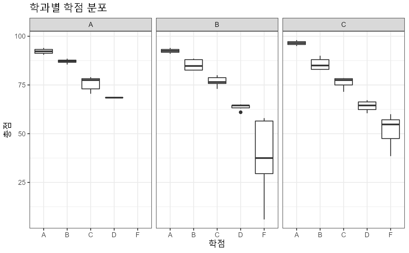

two_grades <- exam_score %>% 
 filter(grade %in% c("A", "F"))

two_grades %>% 
  count(grade)
#> # A tibble: 2 × 2
#>   grade     n
#>   <chr> <int>
#> 1 A         8
#> 2 F        13

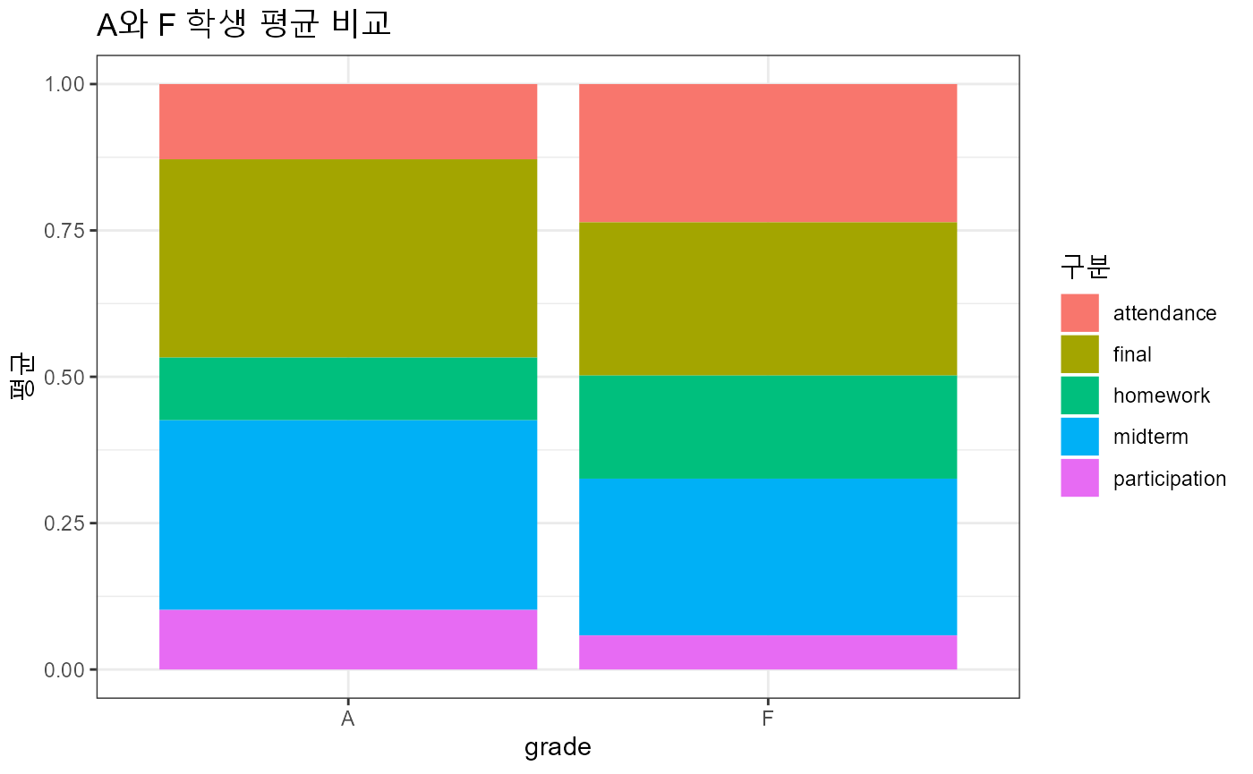
two_grades %>% 
  pivot_longer(cols = attendance:final, 
               names_to = "구분",
               values_to = "점수") %>% 
  group_by(grade, 구분) %>% 
  summarise(평균 = mean(점수)) %>% 
  ggplot(aes(x = grade, y = 평균, fill = 구분)) +
     geom_col(position = "fill") +
     theme_bw(base_family = "AppleGothic") +
     labs(title = "A와 F 학생 평균 비교")
#> `summarise()` has grouped output by 'grade'. You can override using the
#> `.groups` argument.